2829
Application of a Clinically Viable Deep-Learning-Based QSM Workflow on Stroke Cases1Joint Department of Biomedical Engineering, Marquette University and Medical College of Wisconsin, Milwaukee, WI, United States, 2Department of Radiology, Medical College of Wisconsin, Milwaukee, WI, United States
Synopsis
Quantitative Susceptibility Mapping (QSM) can quantitatively estimate tissue magnetic susceptibility, which enables differentiation of diamagnetic calcifications and paramagnetic hemorrhages. The translation of QSM into clinical practice faces technical implementation challenges, particularly the QSM inversion process. In the clinical practice current QSM post-processing techniques are constrained due to large slick thicknesses, which result in compromised background field removal and streaking artifacts in QSM images. To address these limitations, here we a apply a deep-learning-based QSM pipeline, including: (1) a 2D neural network to construct brain masks, (2) a background field removal deep neural network reveal local tissue fields, and (3) a QSM inversion deep neural network. Nine patients with stroke were scanned using a clinical susceptibility-weighted MR protocol were used to demonstrate that the proposed clinically viable QSM workflow can effectively detect microbleeds and differentiate calcifications from hemorrhages.
Purpose
Susceptibility Weighted Imaging (SWI) can effectively detect hemorrhages using susceptibility contrast, but suffers from blooming effects and struggles to differentiate calcifications from microbleeds or iron deposits1. Quantitative Susceptibility Mapping (QSM), in estimating the underlying tissue magnetic susceptibilities, is able to differentiate diamagnetic calcifications from paramagnetic hemorrhages2,3. Current approaches to solve the QSM inverse problem either suffer from spatial streaking artifacts or require long computation times. As a result, QSM clinical translation is hindered. Here, we proposed a deep-learning QSM pipeline, which includes (1) a 2D neural network to construct brain masks, (2) a background field removal deep neural network to reveal local tissue fields, and (3) a QSM inversion deep neural network.Methods
- Datasets: Nine patients with stroke were scanned using a clinical susceptibility-weighted MR protocol on a 3T MRI scanner, with data acquisition parameters: in-plane data matrix = 288x224, FOV = 22 cm, slice thickness = 3.0 mm, parallel imaging factors = 2x1, number of slices = 46-54, number of echoes = 7, echo spacing = 4.1ms, flip angle = 15˚, TR = 39.7ms, total scan time of roughly 2.5 minutes.
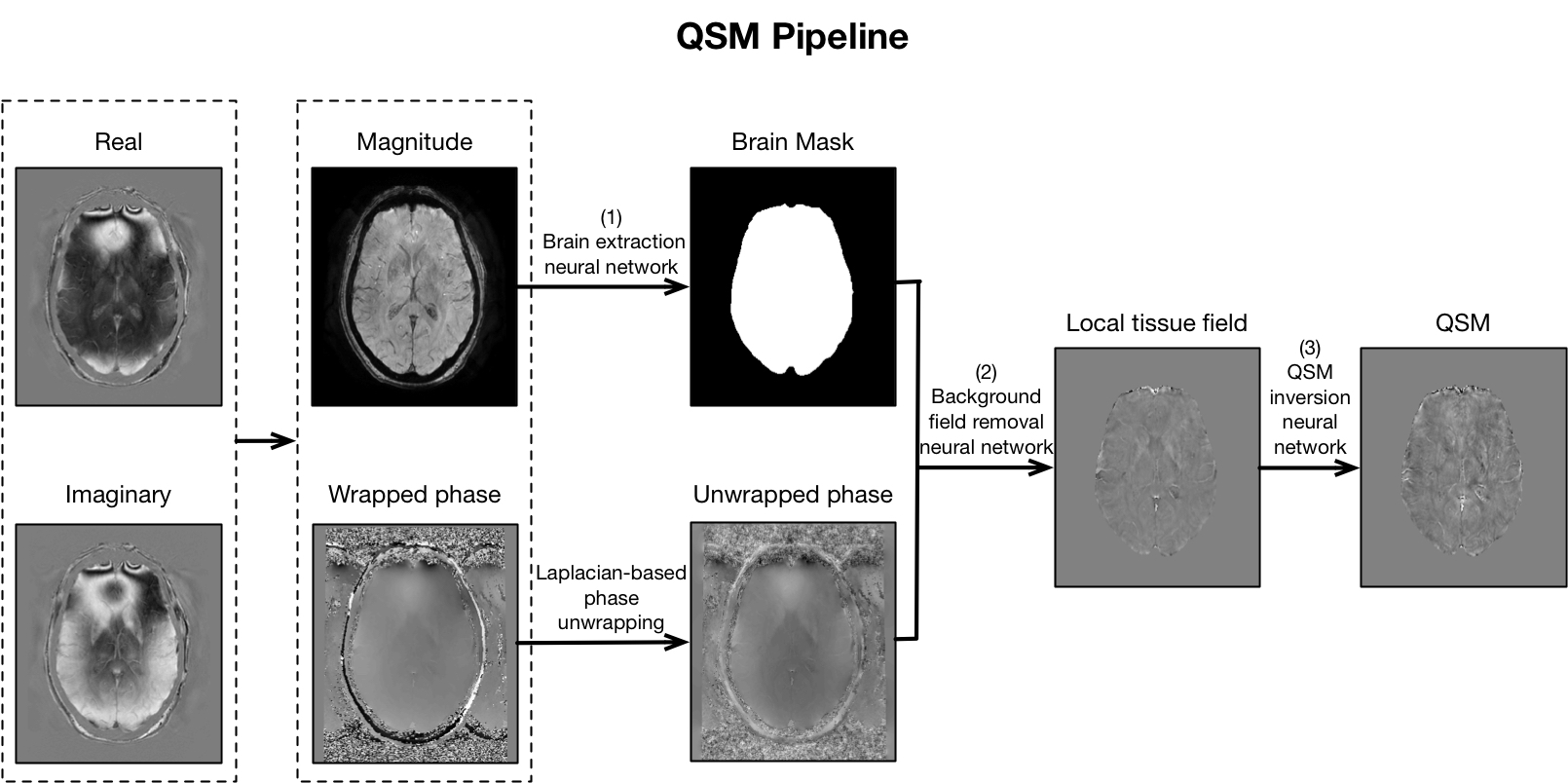
- Data Processing: SWI images were processed by vendor reconstruction algorithms. The raw k-space data were saved for offline QSM processing, which is illustrated in Fig.1. Complex multi-echo images were reconstructed from raw k-space data. The magnitude and phase images were calculated using the real and imaginary images. Laplacian-based phase unwrapping was applied to remove the phase wraps. The brain masks were obtained from the magnitude images using a locally developed brain extraction neural network. Using the unwrapped phase maps and brain masks as inputs, the background removal neural network output the tissue field maps. Finally, our Approximated Susceptibility through Parcellated Encoder-decoder Networks (ASPEN) deep learning model was applied to produce the final susceptibility maps. On conventional CPU hardware, this entire pipeline requires 1-2 minutes, on routine GPU hardware, the pipeline can be performed in seconds.
- Evaluation: The conventional SWI images and corresponding QSM images were evaluated in comparison. For each case, the number of hypointense regions in SWI were manually counted. In the corresponding QSM images, regions of hypointense and hyperintense values, indicating low susceptibility and high susceptibility values, were labeled and counted.
Results and Discussion
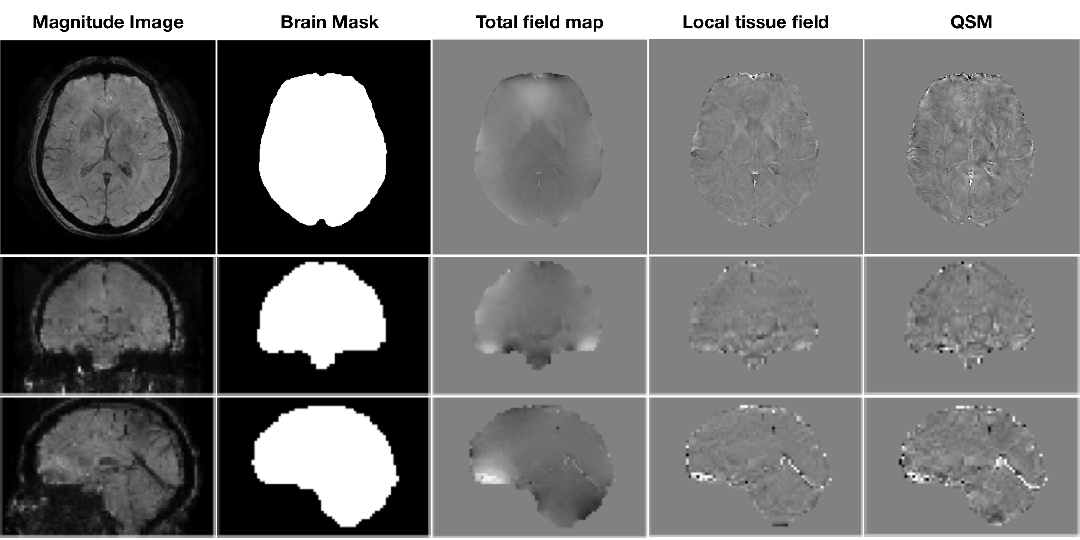
In Fig.2, the data processing results using above methods on one subject are shown in three (axial/coronal/sagittal) views. The local field maps (fourth column) after background removal show homogeneous background removal. QSM images shows high image quality with fine details and negligible streaking artifacts.
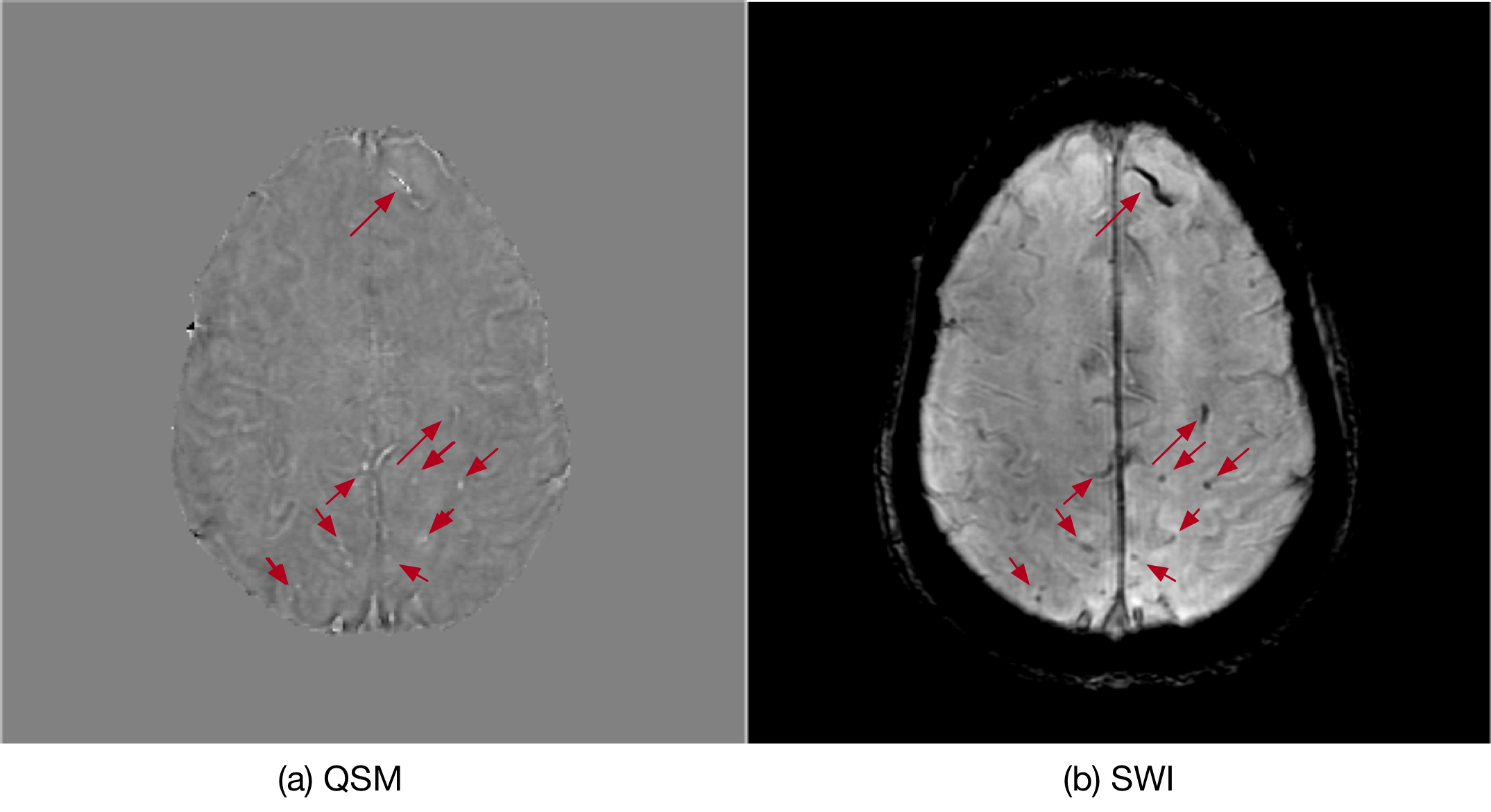
In Fig.3, the SWI and QSM images of one stroke patient are illustrated, where QSM can effectively detect the small microbleeds identified within the SWI images. This indicates that the neural network pipeline is able to produce high quality QSM maps using a routine clinical SWI protocol. Compared to typical research QSM scans, clinical SWI protocols have shorter data acquisition durations (lower resolution) and thicker slice thickness (less isotropic).
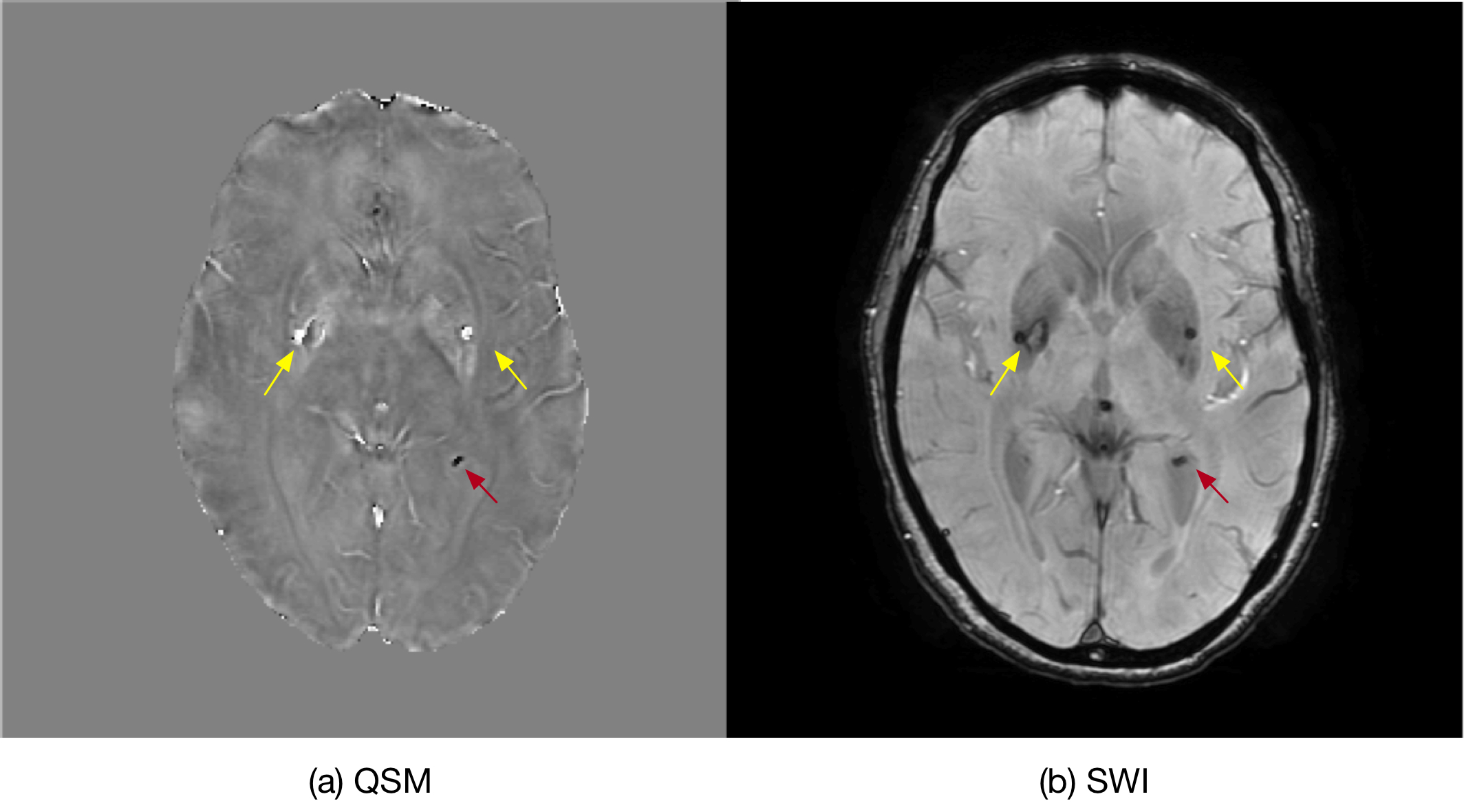
In Fig.4, the SWI and QSM images of one stroke patient are displayed. The cerebral microbleeds and calcifications all appear as black hypointense regions in SWI images, making it difficult to differentiate one from another. In QSM images, microbleeds (paramagnetic) show as bright/hyperintense regions, while calcifications (diamagnetic) are dark/hypointense regions. Therefore, QSM can effectively differentiate calcifications from real microbleeds.
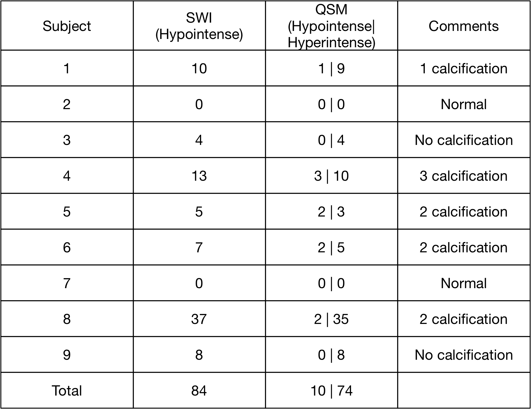
In Table.1, the number of dark/hypointense regions found in SWI images and the number of dark/hypointense or bright/hyperintense regions found in QSM images are summarized. In five stroke patients, dark/hypointense regions were found in SWI and QSM images, indicating they are likely to be calcifications. The crucial finding from this study is that within 9 subjects, a total of 10 hypointense regions in SWI were confirmed using QSM to be calcifications, not microbleeds. This accounts for over 10% of the microbleeds that could have been identified using SWI alone.
Conclusion
A clinically viable deep learning based QSM workflow was demonstrated on a cohort of clinical stroke SWI datasets. The QSM images reconstructed were of sufficient quality to allow for meaningful differential quantification of calcifications and microbleeds. These preliminary results show that clinical use of QSM on stroke patients can improve sensitivity, specificity and allow for more accurate measurements of total lesion load when compared with SWI.Acknowledgements
No acknowledgement found.References
1. Haacke EM, Xu Y, Cheng YCN and Reichenbach JR. Susceptibility weighted imaging (SWI). Magnetic Resonance in Medicine. 2004; 52 (3): 612-618.
2. Wang Y and Liu T. Quantitative susceptibility mapping (QSM): decoding MRI data for a tissue magnetic biomarker. Magnetic resonance in medicine. 2015; 73 (1): 82-101.
3. Chen W, Zhu W, Kovanlikaya I, et al. Intracranial calcifications and hemorrhages: characterization with quantitative susceptibility mapping. Radiology. 2014; 270 (2): 496-505.
Figures