2721
Comparison of Gradient Echo and Gradient Echo Sampling of Spin Echo Sequence for the Quantification of the Oxygen Extraction Fraction by Combining Quantitative Susceptibility Mapping and Blood Oxygenation Level Dependency1Computer Assisted Clincial Medicine, Medical Faculty Mannheim, Heidelberg University, Mannheim, Germany, 2Department of Biomedical Engineering, Cornell University, Ithaca, NY, United States, 3Department of Radiology, Weill Cornell Medical College, New York, NY, United States, 4Department of Radiology, Tongji Hospital, Wuhan, China
Synopsis
The oxygen extraction fraction (OEF) is a promising biomarker for cerebral tissue vitality. Combining quantitative blood oxygenation level-dependent (qBOLD) modelling and quantitative susceptibility mapping (QSM) from gradient echo (GRE) data revealed promising results but still suffered from biases in white matter and required good parameter initialization. We showed that using an additional gradient echo sampling of spin echo (GESSE) sequence enables OEF reconstruction with higher accuracy, precision and robustness to parameter initialization in simulation. Yet, this increased robustness did still not allow for parameter initialization without prior knowledge of local distributions in vivo, which lead to a non-physiological gray-white matter contrast in the OEF.
Introduction
The oxygen extraction fraction (OEF) is a promising parameter for cerebral tissue vitality especially in stroke and brain tumor patients. MRI-based OEF mapping suffers from low signal-to-noise ratio making an accurate reconstruction challenging. Cho et al.1 applied quantitative susceptibility mapping (QSM) to regularize the quantitative blood oxygenation level-dependent (qBOLD) reconstruction of OEF from gradient echo data (GRE) showing promising results. However, it seemed to introduce a bias in white matter and required extensive parameter initialization. Here, we used a gradient echo sampling of spin echo (GESSE) sequence in order to overcome the abovementioned issues and compared it to the original approach for OEF quantification from qBOLD+QSM in simulation and 7 healthy volunteers regarding parameter accuracy, precision and robustness to initialization.Methods
2D-GESSE, 3D-GRE and 2D-EPI pseudo-continuous arterial spin labeling (pCASL) data were acquired from 7 healthy volunteers on a clinical 3T Magnetom TRIO scanner (Siemens Healthineers, Erlangen, Germany). GESSE parameters were: TR$$$\,=\,$$$2780$$$\,$$$ms; TE1$$$\,=\,$$$29$$$\,$$$ms; ΔTE$$$\,=\,$$$2$$$\,$$$ms; 32 echoes; spin echo$$$\,=\,$$$#10; matrix size$$$\,=\,$$$128$$$\,$$$x$$$\,$$$96; 20 slices; voxel size$$$\,=\,$$$2$$$\,$$$x$$$\,$$$2$$$\,$$$x$$$\,$$$2$$$\,$$$mm³; acquisition time$$$\,=\,$$$10:00$$$\,$$$min. GRE parameters were: TR$$$\,=\,$$$61$$$\,$$$ms; TE1$$$\,=\,$$$4.5$$$\,$$$ms; ΔTE$$$\,=\,$$$5.5$$$\,$$$ms; 8 echoes; matrix size$$$\,=\,$$$256$$$\,$$$x$$$\,$$$192$$$\,$$$x$$$\,$$$72; voxel size$$$\,=\,$$$0.9$$$\,$$$x$$$\,$$$0.9$$$\,$$$x$$$\,$$$1.4$$$\,$$$mm³; acquisition time$$$\,=\,$$$7:51$$$\,$$$min. Cerebral blood flow (CBF) was calculated from pCASL data.2 QSM was applied to the GRE data and employed as a regularization for the single-compartment quantitative BOLD fit following the approach of Cho et al.1 to the GESSE and GRE data respectively to quantify OEF, deoxygenated blood volume ν, R2, non-blood susceptibility χnb and signal intensity S0: $$\text{argmin}_{\text{OEF},\nu,R_2,S_0,\chi_\text{nb}}\left[\sum_\text{TE} ||S_\text{GESSE/GRE}(\text{TE}))-F_\text{qBOLD}(\text{OEF},\nu,R_2,S_0,\chi_\text{nb},\text{TE})\}||_2^2\\+w||\text{QSM}-F_\text{QSM}(\text{OEF},\nu,\chi_\text{nb}))||_2^2\right] .$$ FQSM calculates magnetic susceptibility according to Cho et al.1. FqBOLD is the single-compartment qBOLD model for GESSE3,4:$$F_\text{qBOLD}(\text{OEF},\nu,R_2,S_0,\chi_\text{nb},t)=S_0\cdot\text{exp}(-\nu\cdot f(\delta\omega\cdot t)-R_2\cdot(t+\text{SE}))$$ with t being referenced to the time of spin echo SE and GRE (5):$$F_\text{qBOLD}(\text{OEF},\nu,R_2,S_0,\chi_\text{nb},t)=S_0\cdot\text{exp}(-R_2\cdot t)\cdot\left(1-\frac{\nu}{1-\nu}\cdot f(\delta\omega\cdot t)+\frac{1}{1-\nu}\cdot f(\nu\cdot \delta\omega\cdot t)\right)$$ respectively with the hypergeometric function (6):$$f(\delta\omega\cdot t)=~_1F_2\left(\{-0.5\};\{0.75,1.25\};-\frac{9}{16}(\delta\omega\cdot t)^2\right)-1$$ and frequency shift:$$\delta\omega(\text{OEF},\chi_\text{nb})=\frac{1}{3}\cdot\gamma\cdot B_0\cdot\left[\text{Hct}\cdot\Delta\chi_0\cdot(1-\text{SaO2}\cdot(1-\text{OEF}))+\chi_\text{ba}-\chi_\text{nb}\right]\,.$$ The constants are hematocrit7 Hct$$$\,=\,$$$0.357, susceptibility difference between fully de- and oxygenated red blood cells8 Δχ0$$$\,=\,$$$3.481$$$\,$$$ppm, arterial oxygen saturation SaO2$$$\,=\,$$$0.98 and fully oxygenated blood susceptibility9 χba$$$\,=\,$$$-0.1082$$$\,$$$ppm. The parameters were initialized with a fit to low resolution data for GESSE and by estimating OEF from straight sinus and ν from CBF10 and using those values to fit for an initial estimate of S0 and R2 for GRE. The weighting factor was determined with an L-curve approach.11 Intersubject means of the parameters were compared (Student’s t) between sequences within the same tissue type and between tissue types within the same sequence. An 8$$$\,$$$x$$$\,$$$8$$$\,$$$x$$$\,$$$8 voxel single- and multi-compartment simulation representing the three compartments of white matter12 with SNR$$$\,=\,$$$190 was also utilized. The former was performed with optimal and biased ($$$\pm$$$20% OEF and ν), the latter only with optimal initialization. Accuracy and precision were determined as relative bias of the reconstructed mean and relative standard deviation over all voxels respectively.
Results
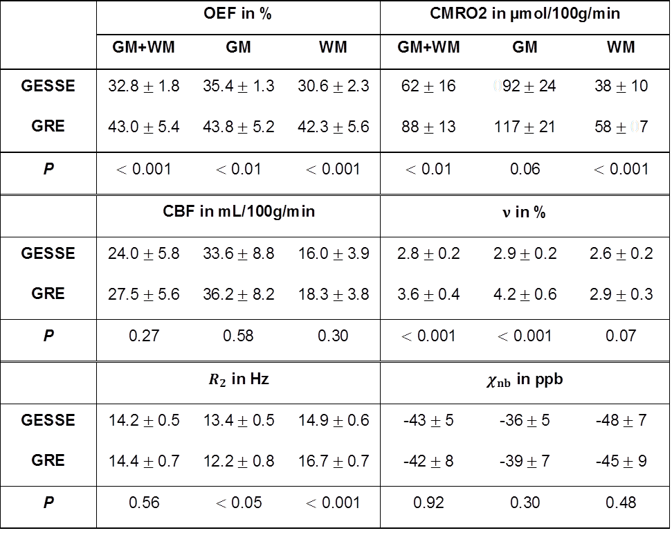
GESSE parameters showed higher accuracy, precision and robustness to initialization in simulation (Table 1). GRE reconstruction slightly overestimated OEF for single-compartment (+6%) and strongly for multi-compartment simulations (+68%) despite optimal initialization. Intersubject means and standard deviations over gray and white matter of the healthy volunteers were OEF$$$\,=\,$$$32.8$$$\,\pm\,$$$1.8$$$\,$$$%, ν$$$\,=\,$$$2.8$$$\,\pm\,$$$0.2$$$\,$$$%, R2$$$\,=\,$$$14.2$$$\,\pm\,$$$0.5$$$\,$$$Hz, χnb$$$\,=\,$$$-43$$$\,\pm\,$$$5$$$\,$$$ppb for GESSE and OEF$$$\,=\,$$$43.0$$$\,\pm\,$$$5.4$$$\,$$$%, ν$$$\,=\,$$$3.6$$$\,\pm\,$$$0.4$$$\,$$$%, R2$$$\,=\,$$$14.4$$$\,\pm\,$$$0.7$$$\,$$$Hz, χnb$$$\,=\,$$$-42$$$\,\pm\,$$$8$$$\,$$$ppb for GRE with a significant difference (P$$$\,<\,$$$0.05) for OEF and ν (Table/Figure 1). Gray-white matter contrast was significant (P$$$\,<\,$$$0.05) in all parameters for GESSE but only in ν and R2 for GRE (Figure 1). Figure 2 depicts a representative slice of reconstructed parameters from GESSE and GRE respectively. Figure 3 illustrates the parameter distribution across gray and white matter for one subject.Discussion
The parameters reconstructed from GESSE showed higher accuracy and precision in simulation due to the more extensive sampling of the signal decay especially around the spin echo. Moreover, they were less sensitive to parameter initialization. The in vivo analysis revealed significantly lower OEF for GESSE with both still being in a physiologically acceptable range.13 Gray-white matter contrast is distributed into all parameters for GESSE but not present in OEF for GRE. The OEF contrast for GESSE disagrees with the uniformity reported in literature.14 The lack of it for GRE, however, is mainly enforced by the chosen way for initialization. ν does not deviate much from the initial guess for GRE making its accuracy and, due to the strong coupling, the accuracy of all parameters highly dependent on this estimate. A comparison with 15O-PET is necessary to determine the exact OEF bias of both methods in vivo.Conclusion
The GESSE sequence outperforms GRE in simulation. Good initialization is, however, still required in vivo so that the improved performance does not outweigh the drawbacks of lower resolution and an additional acquisition. Nonetheless, most effort should be put into obtaining accurate parameter initialization when using GRE based OEF reconstruction.Acknowledgements
No acknowledgement found.References
1. Cho J, Kee Y, Spincemaille P, Nguyen TD, Zhang J, Gupta A, Zhang S, Wang Y. Cerebral Metabolic Rate of Oxygen (CMRO2) Mapping by Combining Quantitative Susceptibility Mapping (QSM) and Quantitative Blood Oxygenation Level-Dependent Imaging (qBOLD). Magn Reson Med 2018. doi: 10.1002/mrm.27135.
2. Alsop DC, Detre JA, Golay X, et al. Recommended implementation of arterial spin-labeled Perfusion mri for clinical applications: A consensus of the ISMRM Perfusion Study group and the European consortium for ASL in dementia. Magn Reson Med 2015;73(1):102-116.
3. Yablonskiy DA. Quantitation of intrinsic magnetic susceptibility-related effects in a tissue matrix. Phantom study. Magn Reson Med 1998;39(3):417-428.
4. Yablonskiy DA, Haacke EM. Theory of NMR Signal Behavior in Magnetically Inhomogeneous Tissues: The Static Dephasing Regime. Magn Reson Med 1994;32:749-763.
5. Ulrich X, Yablonskiy DA. Separation of cellular and BOLD contributions to T2* signal relaxation. Magn Reson Med 2015;615:606-615.
6. Sukstanskii AL, Yablonskiy DA. Theory of FID NMR signal dephasing induced by mesoscopic magnetic field inhomogeneities in biological systems. J Magn Reson 2001;151(1):107-117.
7. Sakai F, Nakazawa K, Tazaki Y, Ishii K, Hino H, Igarashi H, Kanda T. Regional Cerebral Blood Volume and Hematocrit Measured in Normal Human Volunteers by Single-Photon Emission Computed Tomography. J Cereb Blood Flow Metab 1985;5:207-213.
8. Jain V, Abdulmalik O, Propert KJ, Wehrli FW. Investigating the magnetic susceptibility properties of fresh human blood for noninvasive oxygen saturation quantification. Magn Reson Med 2012;68(3):863-867.
9. Zhang J, Zhou D, Nguyen TD, Spincemaille P, Gupta A, Wang Y. Cerebral metabolic rate of oxygen (CMRO2) mapping with hyperventilation challenge using quantitative susceptibility mapping (QSM). Magn Reson Med 2017;77(5):1762-1773.
10. Leenders KL, Perani D, Lammertsma AA, et al. Cerebral blood flow, blood volume and oxygen utilization. Normal values and effect of age. Brain 1990;113(1):27-47.
11. Hansen PC, O'Leary DP. The use of the L-curve in the regularization of discrete ill-posed problems. SIAM J Sci Comput 1993;14(6):1487-1503.
12. Whittall KP, MacKay AL, Graeb DA, Nugent RA, Li DK, Paty DW. In vivo measurement of T2 distributions and water contents in normal human brain. Magn Reson Med 1997;37(1):34-43.
13. He X, Yablonskiy DA. Quantitative BOLD: Mapping of human cerebral deoxygenated blood volume and oxygen extraction fraction: Default state. Magn Reson Med 2007;57(1):115-126.
14. Gusnard DA, Raichle ME. Searching for a Baseline: Functional Imaging and the Resting Human Brain. Nature 2001;2(October):685-694.
Figures