2715

Automatic segmentation of deep grey matter structures for iron quantification

Ying Wang¹, Yongsheng Chen^2,3, David T Utriainen^2,4, and Ewart Mark Haacke^1,2,3,4

¹Biomedical Engineering, Wayne State University, Detroit, MI, United States, ²The MRI Institute for Biomedical Research, Bingham Farms, MI, United States, ³Radiology, Wayne State University, Detroit, MI, United States, ⁴Magnetic Resonance Innovations Inc., Bingham Farms, MI, United States

Synopsis

Quantitative susceptibility mapping (QSM) is a promising iron quantification method for assessing subcortical deep gray matter (SGM) in various neurodegenerative diseases. The accuracy of the measurement depends largely on the accuracy of the structural segmentation. Manually drawn regions-of-interest from a well-trained specialist are often the best but are very time-consuming. In this work, we propose an automatic segmentation method for DGM iron quantification by taking advantage of a hybrid image approach combining T1W images and QSM data. Preliminary results on 5 stroke patients presented an overall 77.8±5.8% Dice coefficient compared to the manually drawn ground truth. The measured susceptibility of the DGM showed good agreement between both methods.

Introduction

Quantitative susceptibility mapping (QSM) is a promising iron quantification method for assessing subcortical deep gray matter (DGM) in various neurodegenerative diseases [1]. The accuracy of the measurement depends largely on the accuracy of the structural segmentation. Manually drawn ROIs from a well-trained specialist are usually the best but are very time-consuming. Atlas-based methods provide a novel approach to deal with structural information [2,3], but typically these methods only use T1W data which often has poor contrast for basal ganglia structures. In this study, we employed a T1W image with enhanced grey matter (GM) to white matter (WM) contrast using a new protocol referred to as STrategically Acquired Gradient Echo (STAGE) imaging [4,5] along with QSM data to get a hybrid image for automated segmentation.

Methods

Data Acquisition: This study was approved by the local IRB. Five stroke patients were recruited and were scanned on a 3T Siemens Trio Tim. The STAGE protocol was used for data acquisition. STAGE generates a number of qualitative and quantitative images, two of which we use in this study: whole brain QSM data and a specially enhanced set of T1W images with improved GM and WM contrast. The latter offers a major advantage in boundary detection for most structures while the former offers good boundaries for iron containing structures such as the Globus pallidus (GP).

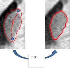
Data processing: There are three major steps to implementing this auto-segmentation approach (Figure 1). Step 1: We generated a 1mm isotropic template from a high quality 3D T1W data set by manually drawing the structures and combining it with the QSM information to ensure reasonable choices for the GP and other basal ganglia structures. We then manually labeled 5 pairs of these structures (Caudate nucleus (CN), Putamen (PUT), GP, Red nucleus (RN), Substantia nigra (SN)). This template data is then mapped to the data for any given individual using a global deformable registration and then, for the CN and PUT, we use a local registration. All patient data are resampled to 1 mm isotropic resolution for this process. Background signal is removed using the automated brain extraction tool (BET) [6]. We chose the Versor3D method with finite processing to do the rigid registration and then performed a B-Splines multi-modality image registration in 3D with ITK [7,8]. We set the node of the B-Spline grid to 5 for global, and 10 for local deformable registration. We used the LBFGSB optimizer which is suitable for a large group of parameters to find the optimal parameters [9, 10]. Finally the data was cropped back to its original form. Step 2: The hybrid image was obtained using the formula: $$$I_{hybrid}=I_{T1WE}-I_{QSM}$$$for segmenting the PUT (Figure 2). For other structures, since density distribution changed between different cases, we use the first step output as the initial region. We calculate the mean value and the standard deviation of each region. Then we set a threshold to remove points not belonging to this structure. Our method is sequence parameter independent. Step 3: Boundary detection with a 3D dynamic programming (DP) centerline driven algorithm [11]. We find the centerline using a morphological skeleton, erosion and opening operation iteratively as follows:

$$S(X)=\bigcup_{r=0}^RS_r(X)$$

$$S_r(X)=X\ominus rB-[(X\ominus rB)\circ drB]$$

where rB is the erosion template, drB is the open template, and $$$(X\ominus rB)$$$ is the erosion on image X. R is the last operation when the image is empty. $$$\ominus$$$ is the erosion operation, and $$$\circ$$$ is the open operation. We already have the initial boundary from previous operations. Then, we update the DP boundary along with the centerline points (Figure 3):

To measure the accuracy of the proposed segmentation methods, the 5 pairs of DGM were manually segmented by two well trained observers, as ground truth; and compared with the automatic segmentation using the Dice coefficient.

Results

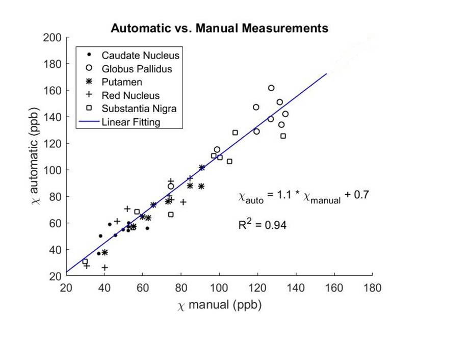
A representative case is shown in Figure 4. Compared to the ground truth, the dice coefficients of the proposed method were 79.4±4.1% for CN, 77.1±5.7% for PUT, 80.8±2.7% for GP, 79.9±6.7 for RN and 71.6±4.6% for SN, respectively. The susceptibility values measured using the automatic segmentation agreed well with those measured manually (Figure 5).

Discussion and Conclusion

Smaller structures resulted in a lower Dice value while larger structures had higher Dice. The measured susceptibility values using the manual masks were lower than those measured automatically, since pixels belonging to the background tissue were included in the manual masks more than the automated masks. However, the overall measured susceptibilities were consistent between manual and automatic measurements. In conclusion, we developed an automatic segmentation algorithm for DGM which can benefit both research and clinical utility.

Acknowledgements

No acknowledgement found.

References

[1] Haacke EM, Liu S, Buch S, Zheng W, Wu D, Ye Y. Quantitative susceptibility mapping: current status and future directions. Magn Reson Imaging 2015;33:1–25. doi:10.1016/j.mri.2014.09.004.

[2] Fischl, B., Salat, D.H., Busa, E., Albert, M., Dieterich, M., Haselgrove, C., van der Kouwe, A.,Killiany, R., Kennedy, D., Klaveness, S., Montillo, A., Makris, N., Rosen, B., Dale, A.M.,2002. Whole brain segmentation: automated labeling of neuroanatomical structures in the human brain. Neuron 33, 341–355.

[3] Fischl, B., Salat, D.H., van der Kouwe, A.J.W., Makris, N., Ségonne, F., Quinn, B.T., Dale, A.M.,2004. Sequence-independent segmentation ofmagnetic resonance images. Neuroimage 23 (Suppl. 1), S69–S84. http://dx.doi.org/10.1016/j.neuroimage.2004.07.016.

[4] Chen Y, Liu S, Wang Y, Kang Y, Haacke EM. STrategically Acquired Gradient Echo (STAGE) imaging, part I: Creating enhanced T1 contrast and standardized susceptibility weighted imaging and quantitative susceptibility mapping. Magn Reson Imaging 2018;46:130–9. doi:10.1016/j.mri.2017.10.005.

[5] Wang Y, Chen Y, Wu D, Wang Y, Sethi SK, Yang G, et al. STrategically Acquired Gradient Echo (STAGE) imaging, part II: Correcting for RF inhomogeneities in estimating T1 and proton density. Magn Reson Imaging 2018;46. doi:10.1016/j.mri.2017.10.006.

[6] Smith SM. Fast robust automated brain extraction. Hum Brain Mapp 2002;17:143–55. doi:10.1002/hbm.10062.

[7] Unser M. Splines: A perfect fit for signal processing. Eur. Signal Process. Conf., vol. 2015–March, 2000. doi:10.1109/79.799930.

[8] Wang Y, Zhao H, Kang Y, Haacke EM. Improved tensor based registration: An heterogeneous approach. 2012 IEEE Int. Conf. Inf. Autom. ICIA 2012, 2012, p. 486–90. doi:10.1109/ICInfA.2012.6246855.

[9] R. H. Byrd, P. Lu, and J. Nocedal. A limited memory algorithm for bound constrained optimization. SIAM Journal on Scientific and Statistical Computing, 16(5):1190–1208, 1995. 8.11

[10] C. Zhu, R. H. Byrd, and J. Nocedal. L-bfgs-b: Algorithm 778: L-bfgs-b, fortran routines for large scale bound constrained optimization. ACM Transactions on Mathematical Software, 23(4):550–560, November 1997. 8.11

[11] Jing Jiang, Haacke EM, Ming Dong. Dependence of Vessel Area Accuracy and Precision As a Function of MR Imaging Parameters and Boundary Detection Algorithm, JOURNAL OF MAGNETIC RESONANCE IMAGING 25:1226–1234 (2007)

Figures

Figure 1. Data processing flowchart. The THA and PT structures are well defined with conventional T1W, however the STAGE enhanced T1W (CN) and QSM images (RN, SN, GP), as well as their hybrid image (PUT), are used to create additional contrast for improved segmentation as iron content and T1 mapping values can aid in differentiating them from surrounding background tissue.

Figure 2. 1st row is the ROI of PUT with STAGE T1W images, 2nd row is the response hybrid images. The addition of the contrast from QSM due to the structures increased iron content dominance relative to surrounding structures allows for increased contrast and improved segmentation.

Figure 3. DPC boundary detection, the left image shows the initial boundary with the centerline and the right image shows the final boundary.

Figure 4. Representative images demonstrating the results for segmenting deep grey matter structures.

Figure 5. Susceptibility values for all five structures comparing between manual and automatic methods. The linear fitting shows a good agreement between both methods for iron quantification.

Proc. Intl. Soc. Mag. Reson. Med. 27 (2019)

2715