2510
Protocol for multi-site quantitative evaluation of 13C radio frequency coils1GE Healthcare, Dallas, TX, United States, 2GE Healthcare, Munich, Germany, 3UT Southwestern Medical Center, Dallas, TX, United States, 4Technical University of Denmark, Kongens Lyngby, Denmark, 5GE Healthcare, Toronto, ON, Canada
Synopsis
We present a protocol for measurement of SNR profile of 13C RF coils for clinical imaging systems. This protocol makes use of standard, vendor-provided pulse sequences as well as the natural abundance 13CH3 resonance of the dimethyl silicone (DMS) phantoms which are widely distributed. We also provide an open source code for processing and analysis.
Introduction
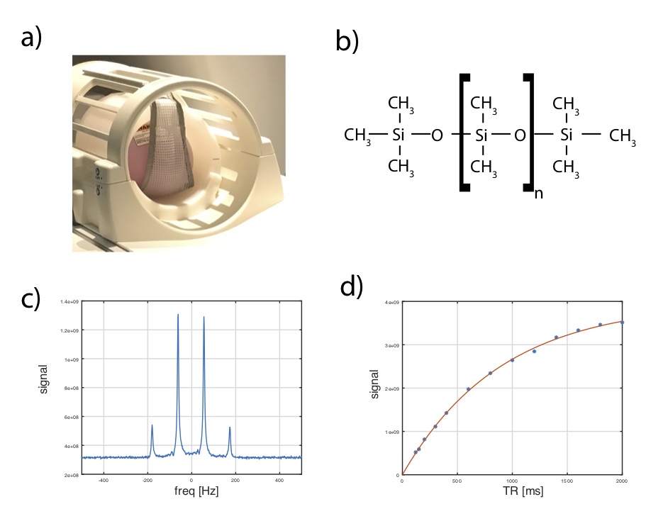
Quantitative comparison of the performance of MRI transmitters and receivers between sites is critically important in establishing standards for performance, selecting appropriate coil geometry for a given application, and verifying hardware reliability for clinical trials. Comparing 13C coils is inherently difficult due to the lack of availability of standardized 13C phantoms, pulse sequences, and data reconstruction and analysis tools. Furthermore, material costs for 13C – enriched compounds for large volume phantoms is prohibitively expensive, and a consensus has not been reached for the selection of the appropriate compound. Developing multi-site studies will be important in the evolution of hyperpolarized 13C technology. We propose here a solution using standard pulse sequences and MRI phantoms, that are widely available. The proposed QA protocol utilizes the natural abundance 13CH3 resonance of the dimethyl silicone (DMS) phantoms available as a QA phantom from some vendors or easily prepared [1] (Figure 1). This phantom has a measured 13C T1 of 899 ms at 3T by saturation recovery, and 13C - 1H coupling constant is measured to be J=118Hz (Figure 1). Compared to the commonly used natural abundance ethylene glycol 13CH2 resonance for phantom calibration, DMS resonates at 62 PPM lower frequency with approximately 50% less sensitivity. Pulse sequence and parameters are discussed, and an open source data reconstruction framework is provided.Methods
Pulse Sequence: The following list gives the relevant parameters of this acquisition protocol. Flip angle calibration was performed manually by finding the null of the resonance using a 3 second TR. A separate protocol was developed for head and torso array testing; this was to ensure that the pixel volume compensated the reduced sensitivity of the larger coils, and to ensure that the FOV sufficiently encompassed a noise region. A 2D phase-encoded, slice-selective spectroscopy sequence was selected since the protocol resolved the spectral splitting without generating image blurring, and noise and signal separation could be achieved by simple band selection in post processing.
- FOV = 32 cm (head), 48 cm (torso)
- acquisition size = 16 by 16
- slice thickness = 2 cm (head), 3 cm (torso)
- averages = 2
- TR = 500 ms
- flip angle = 22.5
- bandwidth, samples = 5 kHz, 256
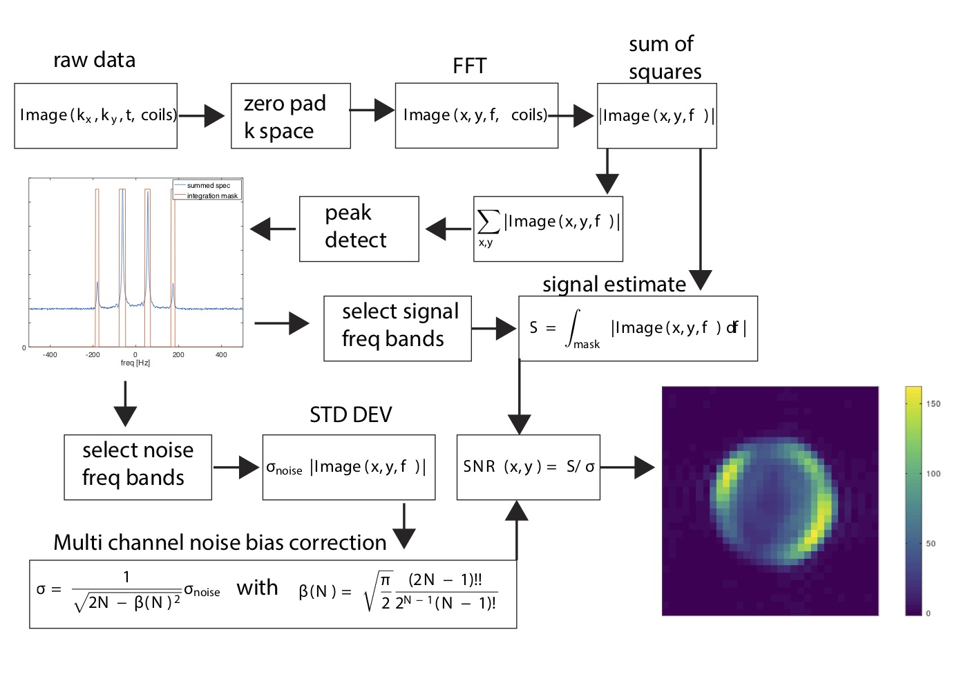
Data processing: Figure 2 shows a schematic of the processing pipeline. Since the A/D period is spectroscopically resolved, signal and noise contributions may be differentiated via band selection. A convenient method is peak selection using the Dietrich method, which relies on computing a numerical derivative, converting to power spectrum, then iterative thresholding based on mean and standard deviations. References [2,3] provide a detailed description of this method, and 1D erosion / dilation morphology operations may be applied to clean up noise spikes. The integration of peaks selected with this method provides maximally efficient signal usage while minimizing noise bias. Since the noise statistics are calculated after performing a sum-of-squares operation, the standard deviation must be corrected for the non-central chi distribution statistics that describe summing multiple channels of Rician-distributed magnitude noise [4,5]. Source code, written in Octave, is openly distributed at the following link [6].
Experiments: This protocol was applied at 3 different sites in the US and Canada using GE 3T Signa systems (GE Healthcare, Waukesha WI) using 3 different 13C array geometries: 8 channel receive array, quadrature birdcage transmit / receive, and clamshell Helmholtz transmit, 8 channel paddle array receive.
Results
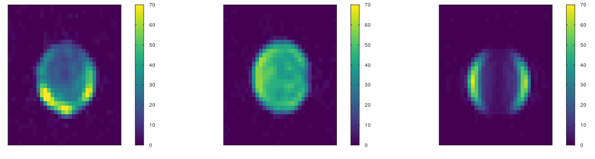
Figure 3 shows 3 sample images acquired with this protocol on the head-sized phantom. In each case, a clear profile of the in-plane SNR behavior of the coil could be achieved, with regions of SNR>50, and scan times under 5 minutes. Figure 3a and 3b show data from an 8 channel receive array and birdcage, respectively. The brightening of the posterior array elements indicates the phantom was more proximal to the posterior side, while the birdcage has smaller inner diameter and thus more even SNR throughout the volume.Discussion / Conclusion
We present a standardized calibration procedure for receive arrays using readily available phantoms and pulse sequences and using open source data processing. Limitations of this protocol include the inherent difficulty in transmit gain determination and lack of robust automated prescan, which obviously may lead to systematic bias of SNR measurements. The effect of coil loading on SNR measurements must be explored further. Although the DMS phantoms are impervious to standing wave effects at high field [1], they are not, by default, loaded and are typically used in conjunction with a cylindrical loading ring (Figure 1). This ring is compatible with most 13C torso arrays, but the smaller head-sized loader is not mechanically compatible with many head arrays. Further study is required to test the adequacy of saline bags for this purpose.Acknowledgements
No acknowledgement found.References
- Skloss T. Phantom Fluids for High Field MR Imaging. Proc. Intl. Soc. Mag. Reson. Med. 11 (2004)
- Cobas JC, Bernstein MA, Martín-Pastor M, Tahoces PG. A new general-purpose fully automatic baseline-correction procedure for 1D and 2D NMR data. J Magn Reson. 2006 Nov;183(1):145-51
- Dietrich W, Rudel CH, and Neumann M. Fast and precise automatic baseline correction of one- and two-dimensional NMR spectra, J. Magn. Reson. 91 (1991) 1–11.
- Gilbert G. Measurement of Signal-to-Noise Ratios in Sum-of-Squares MR Images. J Magn Reson Imaging. 2007 Dec;26(6):1678; author reply 1679.
- Constantinides CD, Atalar E, McVeigh ER. Signal-to-noise measurements in magnitude images from NMR phased arrays. Magn Reson Med 1997:38:852–857.
- https://github.com/galenreed/C13PhantomSNRProtocol.
Figures