2476
Comparison of Reconstruction Methods for Compressed Sensing phosphorus 31P-MRSI1School of Biomedical Engineering, McMaster University, Hamilton, ON, Canada, 2Imaging Research Center, St. Joseph's Healthcare, Hamilton, ON, Canada, 3Electrical and Computing Engineering, McMaster University, Hamilton, ON, Canada
Synopsis
Phosphorus MR spectroscopy and spectroscopic imaging (31P-MRS/MRSI) provide information about energy metabolism, membrane degradation and pH in vivo. However, these methods are not often used primarily because of excessive scan time. Recently, compressed sensing has awakened interest as an acceleration method for MR signal acquisition. In this work we present a 31P-MRSI sequence that combines a flyback-EPSI trajectory with compressed sensing, and we compared two reconstruction methods, conjugate gradient L1-norm minimization and low-rank Hankel matrix completion. Overall, our results showed good preservation of spectral quality for low acceleration factors and an improved performance with the low-rank approach.
Introduction
Phosphorus MR spectroscopy and spectroscopic imaging (31P-MRS/MRSI) provide information about energy metabolism. These methods have been applied in the study of healthy and disease conditions in muscle1 and brain2,3. However, they are not often used primarily because of excessive scan time. To accelerate the acquisition, methods such as EPSI4,5, spiral6 and compressed sensing (CS)7,8 have shown promising results. Under the CS framework, the purpose of this study was to analyze and compare two reconstruction methods, applied to 31P-MRSI data. The first was the CS reconstruction first proposed by Lustig et al.9 (conjugate-gradient L1norm minimization, CGL1) and the second, the low-rank Hankel matrix completion (LR) recently presented by Qu et al.10.Methods
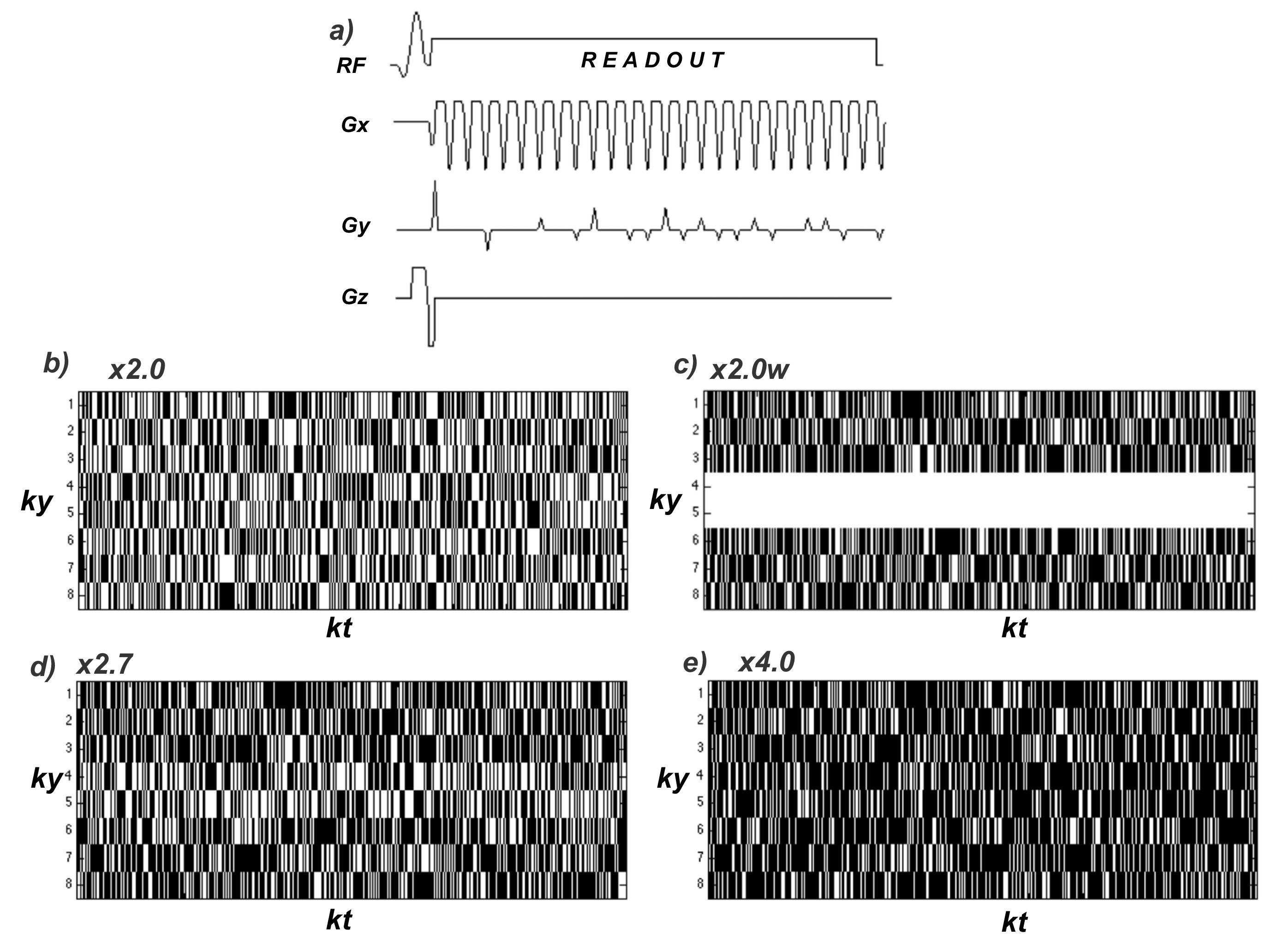
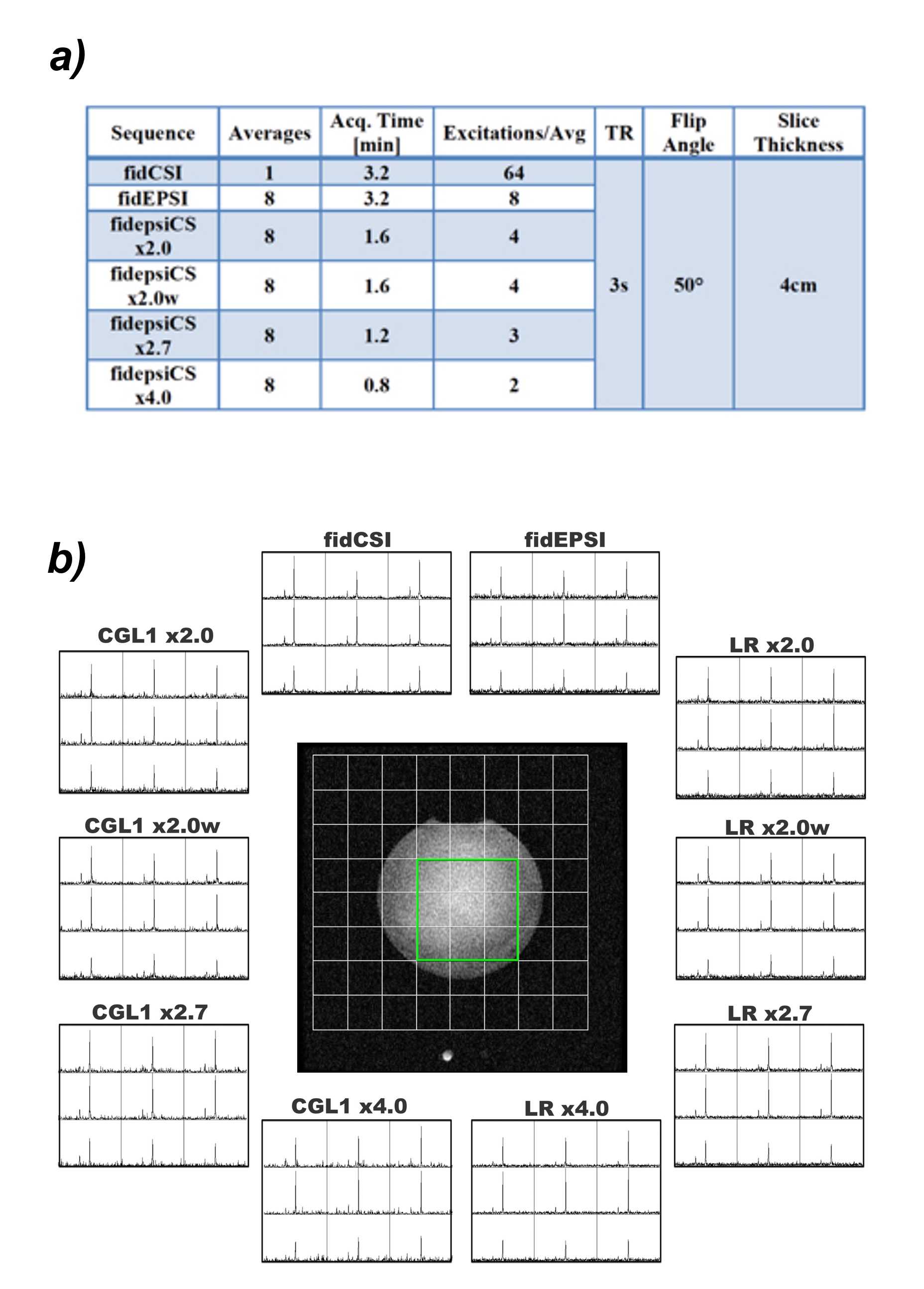
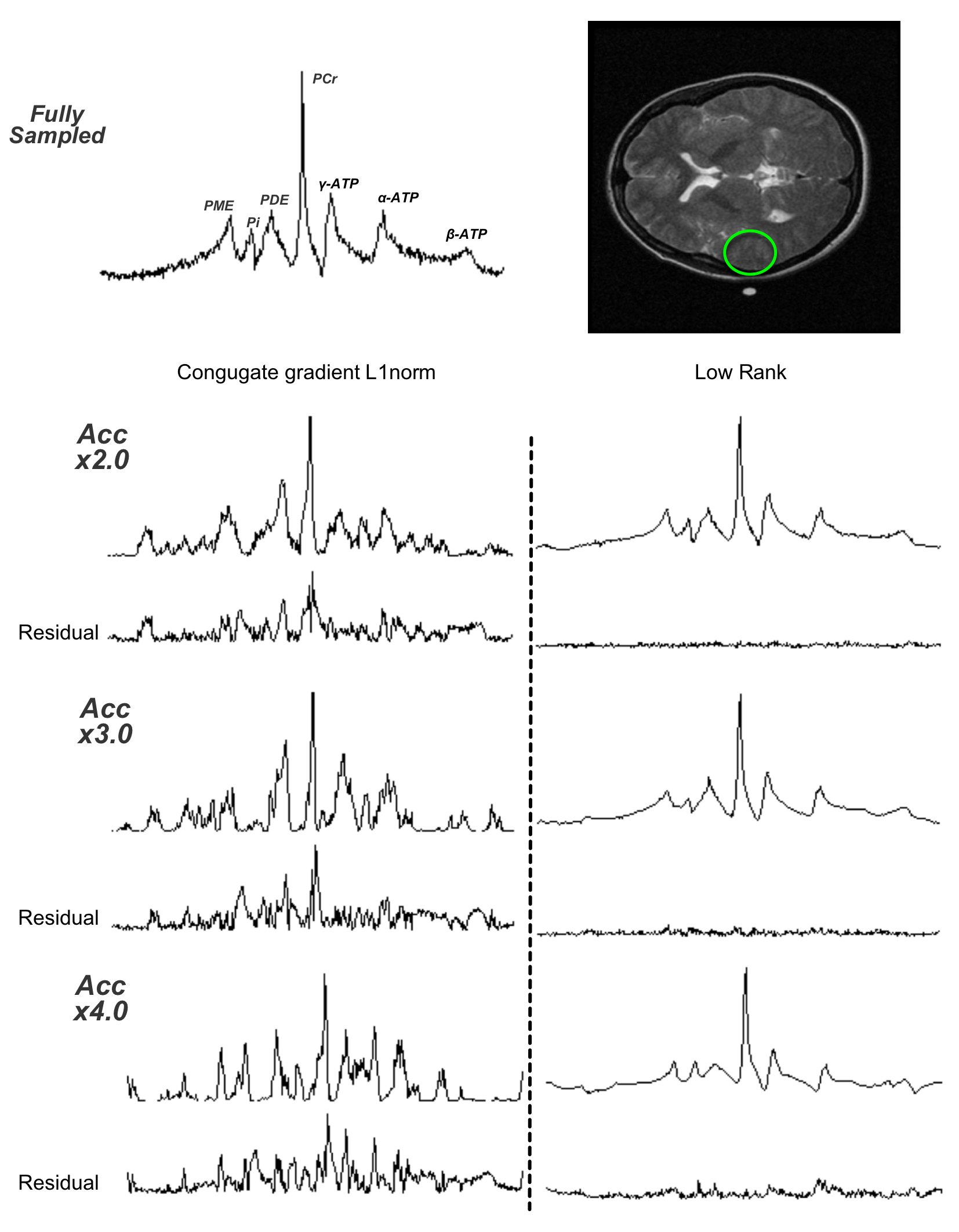
Experiments were performed using a 3T GE-MR750 (GE Healthcare, Milwaukee, WI) scanner and a home-developed pulse sequence built on a flyback-EPSI sequence4. Non-uniform undersampling was achieved by the inclusion of pseudo randomly distributed blips in the ky dimension during the flyback readout to allow sampling multiple kt-ky lines during the same phase encoding step, similar to Hu et al.11,12. Four different schemes were implemented to achieve acceleration factors ranging from 2x-4x (fig.1). The flyback-EPSI trajectory was designed to achieve 2.75x2.75cm2 resolution over a 22x22cm2 field of view (i.e. 8x8 voxels), spectral bandwidth of 1428Hz and 512 points. The pulse sequence (diagram and sub-sampling schemes in fig.1) was tested using an in house designed/built 24cm diameter quadrature birdcage coil tuned to 51.72MHz and a custom-built spherical phantom (volume=1L, pH=6.7) containing 25mmol/L and 10mmol/L sodium phosphate (P1) and phosphocreatine disodium salt (P2), respectively. Six 2D-MRSI datasets were collected using phase encoded MRSI (fidCSI), flyback-EPSI (fidEPSI) and each variation of flyback-EPSI combined with CS (fidepsiCS). Acquisition parameters are shown in fig.2a. Additionally, to test the algorithms using in vivo data, a single fully sampled spectrum was acquired from the parietal lobe of 5 healthy volunteers using a 12.7cm diameter surface coil (51.705MHz), a pulse-acquire sequence, 60° flip angle, 2000Hz spectral bandwidth, 512 points and 128 averages. The collected FIDs were retrospectively under-sampled (pseudo-randomly selected samples) using 256(x2.0), 170(x3.0) and 128(x4.0) data points to match the acceleration factors of fidepsiCS, then spectra were reconstructed using 1D implementations of the algorithms13. Data reconstruction was performed using MATLAB R2015b. Data was re-shaped from the raw blipped acquisition to a 3D matrix of k-space data with dimensions kt-kx-ky, and used as the input for both reconstruction methods. Then, CGL1 reconstruction was performed as follows: (1) data was inverse Fourier transformed in the fully sampled dimension (kx) to convert the problem to multiple 2D reconstructions, then (2) missing kt-ky points were filled using the non-linear conjugate gradient algorithm adapted from the sparseMRI toolbox9; (3) The forward Fourier transform was applied in the kx dimension; and finally (4)data was 3D Fourier transformed. The sparsifying transformation was a 1D length-4 Daubechies Wavelet transform. For the LR reconstruction, data were (1) reordered as a vector containing the FID information for each undersampled kt-ky plane; (2) each vector was used to build a Hankel matrix, feeding into an alternating direction minimization method; (3) reconstructed FIDs were reshaped back into a kt-kx-ky array of data that was (4) Fourier transformed to achieve the 3D-MRSI dataset. To compare performance, in the phantom experiments we selected a 3x3 region of voxels and measured metabolite amplitudes and linewidths. For the in vivo data, metabolite ratios and error (RMSE) were measured and compared to fully sampled results. Data fitting was performed using the OXSA toolbox14.Results
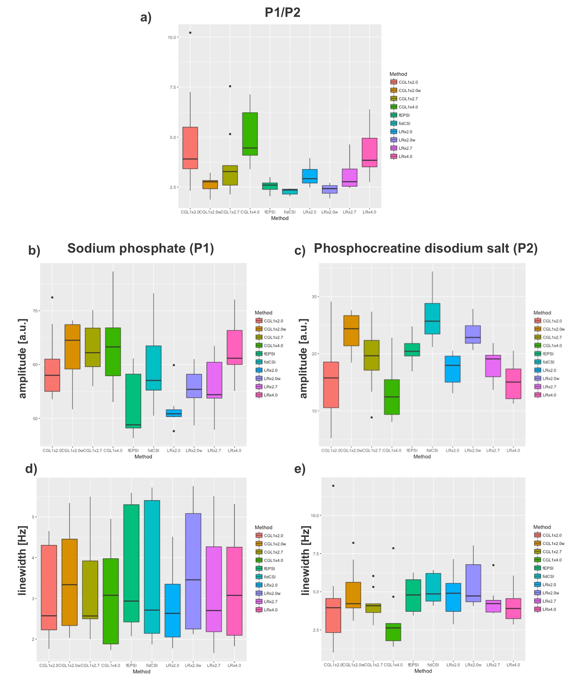
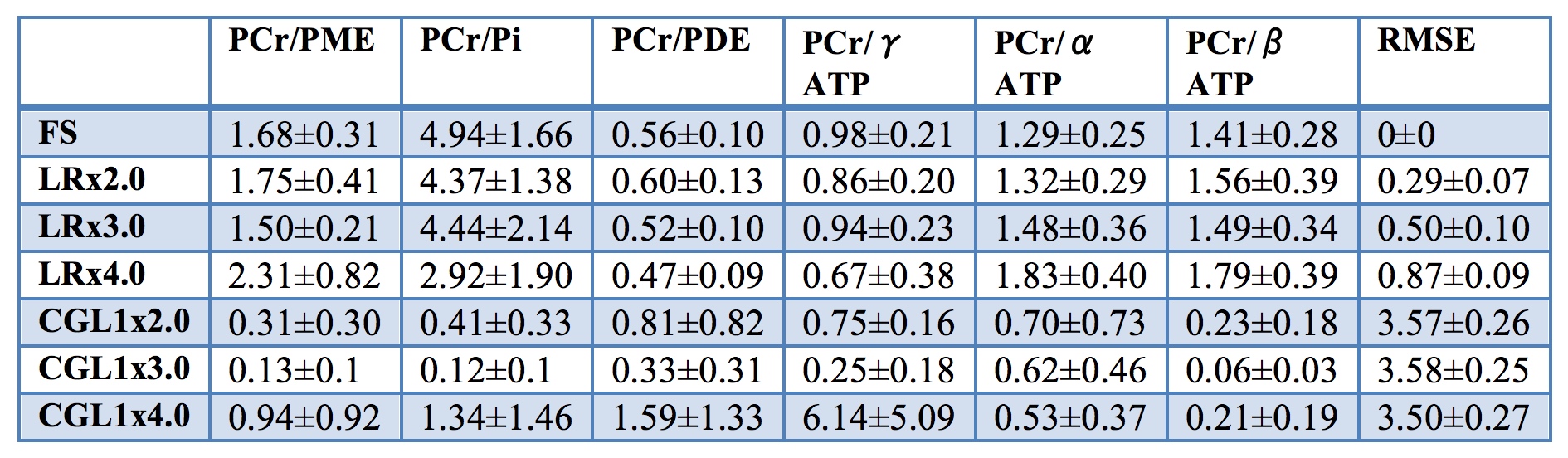
Fig.2b shows a 3x3 voxel region and a comparison of spectra acquired using fidCSI, fidEPSI and all variants of fidepsiCS. Fitted phantom peak amplitudes and linewidths are shown in fig.3. Overall, there was an increase in the P1/P2 ratio for higher accelerations in both methods, however this overestimation was more accentuated for the CGL1 reconstruction. From in vivo acquisitions, it is clear that the CGL1 algorithm failed the reconstruction, as seen in results from fig.4 and fig.5. On the other hand, the LR algorithm performed well.Discussion
We compared two CS reconstruction algorithms applied to 31P-MRSI. From the phantom data, the LR algorithm performed better than CGL1 as depicted by the reduced artifacts shown in the spectra of fig.2 and the plots in fig.3, where fitted values for LR remain comparable to fully sampled fidEPSI up to the x2.7 acceleration. Superiority of the LR algorithm is further demonstrated in our in vivo results.Conclusion
We presented a 31P-MRSI pulse sequence that combines a flyback-EPSI readout with CS and compared two reconstruction algorithms. Our results suggest superiority of the low-rank approach.
Acknowledgements
Funding was provided through a CONACYT (Mexico) scholarship granted to ASD (CVU: 304930) and a NSERC Discovery Grant (RGPIN-2017-06318) to MDN.References
- Valkovič L, Chmelík M, et al. In-vivo 31P-MRS of skeletal muscle and liver: A way for non-invasive assessment of their metabolism. Anal Biochem. 2017;529:193-215.
- Novak J, Wilson M, et al. Clinical protocols for 31P MRS of the brain and their use in evaluating optic pathway gliomas in children. Eur J Radiol. 2014;83(2):e106-e112.
- Harper DG, Jensen JE, et al. Phosphorus spectroscopy (31P MRS) of the brain in psychiatric disorders. eMagRes. 2016;5(2):1257-1270.
- Santos-Díaz A, Obruchkov SI, et al. Phosphorus magnetic resonance spectroscopic imaging using flyback echo planar readout trajectories. Magn Reson Mater Physics, Biol Med. 2018, 31(4):553-564.
- Korzowski A, Bachert P. High-resolution31P echo-planar spectroscopic imaging in vivo at 7T. Magn Reson Med. 2018;79(3):1251-1259.
- Valkovic L, Chmelik M, et al. Dynamic 31P MRSI using spiral spectroscopic imaging can map mitochondrial capacity in muscles of the human calf during plantar flexion exercise at 7T. NMR Biomed. 2016;29(12):1825-1834.
- Hatay GH, Yildirim M, et al. Considerations in applying compressed sensing to in vivo phosphorus MR spectroscopic imaging of human brain at 3T. Med Biol Eng Comput. 2017;55(8):1303-1315.
- Ma C, Clifford B, et al. High-resolution dynamic 31P-MRSI using a low-rank tensor model. Magn Reson Med. 2017;78(2):419-428.
- Lustig M, Donoho D, et al. Sparse MRI: The application of compressed sensing for rapid MR imaging. Magn Reson Med. 2007;58(6):1182-1195.
- Qu X, Mayzel M, et al. Accelerated NMR spectroscopy with low-rank reconstruction. Angew Chemie - Int Ed. 2015;54(3):852-854.
- Hu S, Lustig M, et al. Compressed sensing for resolution enhancement of hyperpolarized 13C flyback 3D-MRSI. J Magn Reson. 2008;192(2):258-264.
- Hu S, Lustig M, et al. 3D compressed sensing for highly accelerated hyperpolarized 13C MRSI with in vivo applications to transgenic mouse models of cancer. Magn Reson Med. 2010;63(2):312-321.
- Shchukina A, Kasprzak P, et al. Pitfalls in compressed sensing reconstruction and how to avoid them. J Biomol NMR. 2016;68(2):79-98.
- Purvis LAB, Clarke WT, et al. OXSA: An open-source magnetic resonance spectroscopy analysis toolbox in MATLAB. PLoS One. 2017;12(9):e0185356.
Figures