2473
Comparison of Spatial Interpolation and Inpainting Methods for Estimation of Bad Fittings in Chemical Shift Imaging Data1Athinoula A. Martinos Center for Biomedical Imaging, Department of Radiology, Massachusetts General Hospital and Harvard Medical School, Charlestown, MA, United States
Synopsis
Chemical Shift Imaging (CSI) allows for the quantification of brain metabolite concentrations across multiple voxels/slices. However, issues with model fit (e.g., suboptimal standard deviation, line width/full width at half-maximum, and/or signal-to-noise ratio) can result in the significant loss of usable voxels. Here, we show that an image restoration method called “inpainting” can be successfully used to restore poorly fitted CSI voxels. This method exhibits superior performance (lowest root-mean-square errors) compared to more traditional methods. Inpainting and similar techniques can prove particularly useful as a means of minimizing voxel loss in group voxelwise analyses in standard space.
Introduction
MR Chemical Shift Imaging (CSI), as opposed to single-voxel-spectroscopy, allows for the quantification of brain metabolite concentrations across multiple voxels/slices, and thus the possibility to perform group voxelwise analyses in standard space. However, for a CSI voxel to be considered viable, it needs to meet several minimum quality-control (QC) criteria, based on the standard deviation of the estimators, the linewidth or full width at half-maximum (FWHM) of their spectrum, and/or the signal-to-noise ratio (SNR). When a voxel is excluded in a participant after QC, the corresponding voxel in all other participants has to be excluded as well, potentially leading to a swiss-cheese-like appearance of the common voxelwise search volume. In this work, we propose the use of an image restoration technique called inpainting1 to help inferring poorly fitted CSI voxels. In order to evaluate the dependency of the inpainting results from contrast type and spatial resolution, we also applied the same technique to high-resolution T1-weighted images. We compared the results using inpainting with those using several, more traditional interpolation methods.Methods
Datasets: 18 healthy controls underwent MR imaging in a 3T Siemens TIM Trio scanner using an 8-channel head and neck coil. MR imaging included an anatomical T1-weighted volume (MEMPRAGE; TR/TE1/TE2/TE3/TE4=2530/1.64/3.5/5.36/7.22ms, flip angle=7º, voxel size=1x1x1mm, acquisition matrix=280x280x208), and chemical shift imaging data (CSI, using LASER excitation and stack-of-spiral 3D k-space encoding; TR/TE=1500/30ms, voxel size=10x10x10mm)2.
LCModel Fitting: Metabolites from CSI data were fitted with LCModel3 and metabolic maps were constructed using MINC/FSL/Matlab tools.
Image Inpainting: Image inpainting, commonly used in art restoration, is a technique used to change an image in a non-detectable form. For the purpose of its application to brain imaging, we have assessed an implementation based on a penalized least squares method that allows restoring missing data by means of the discrete cosine transform4. This method is sometimes also called “fill in”, because it consists of filling in regions presenting problems with the information of the surrounding (either local or non-local) areas.
Multivariate Interpolation Methods: As comparators, we have also used three different multivariate interpolation methods commonly used in medical imaging: nearest neighbor, trilinear and tricubic interpolation. Nearest neighbor interpolation is a simple method that replaces the value of the poorly-fitted voxel with that of the closest neighboring voxel. Trilinear interpolation estimates missing values by fitting f(x)=ax1x+ay1y+az1z+a0. Tricubic interpolation estimates missing values by fitting f(x)=ax3x3+ay3y3+az3z3+ax2x2+ay2y2+az2z2+ax1x+ay1y+az1z+a0, where ax3, ay3, az3, ax2, ay2, az2, ax1, ay1, az1 and a0 are the coefficients of the polynomial, and x, y, and z correspond to points in the space.
Analysis: High-resolution T1-weighted images and N-acetylaspartate (NAA) CSI images (which did not have a significant amount of poorly-fitted voxels) were corrupted to lose a fixed percentage of random voxels, from a 5% to 95% (in steps of 5%). Quantitative performance of the different methods was assessed by comparing the root mean square error (RMSE) computed between ground truth images and interpolated/inpainted images, using a repeated measures analysis of the variance (ANOVA).
Results
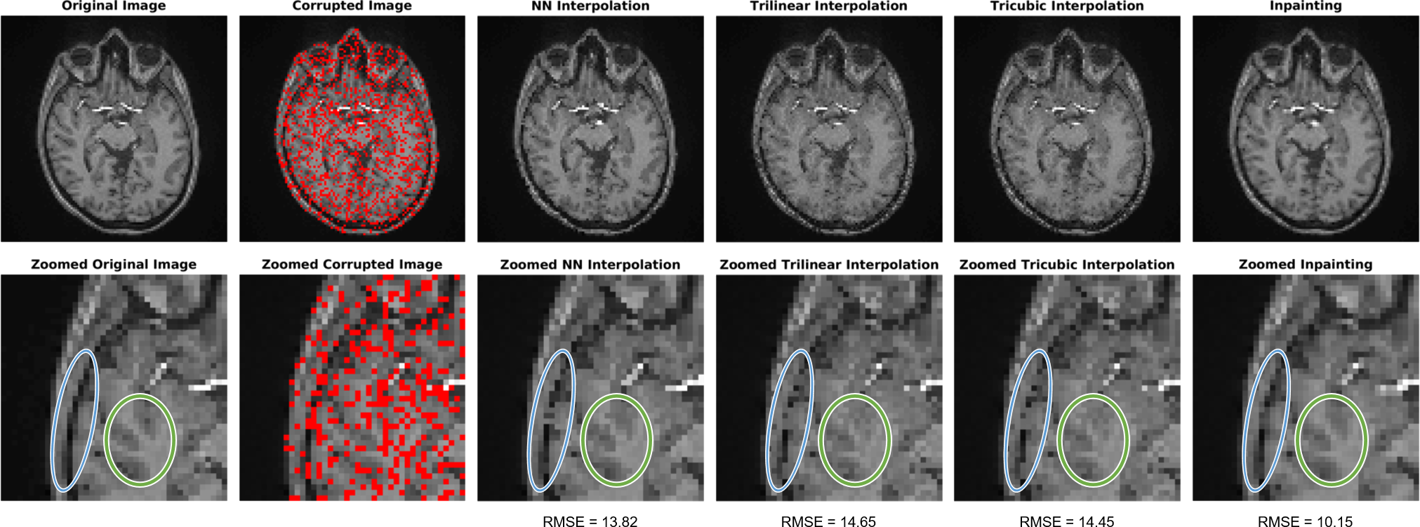
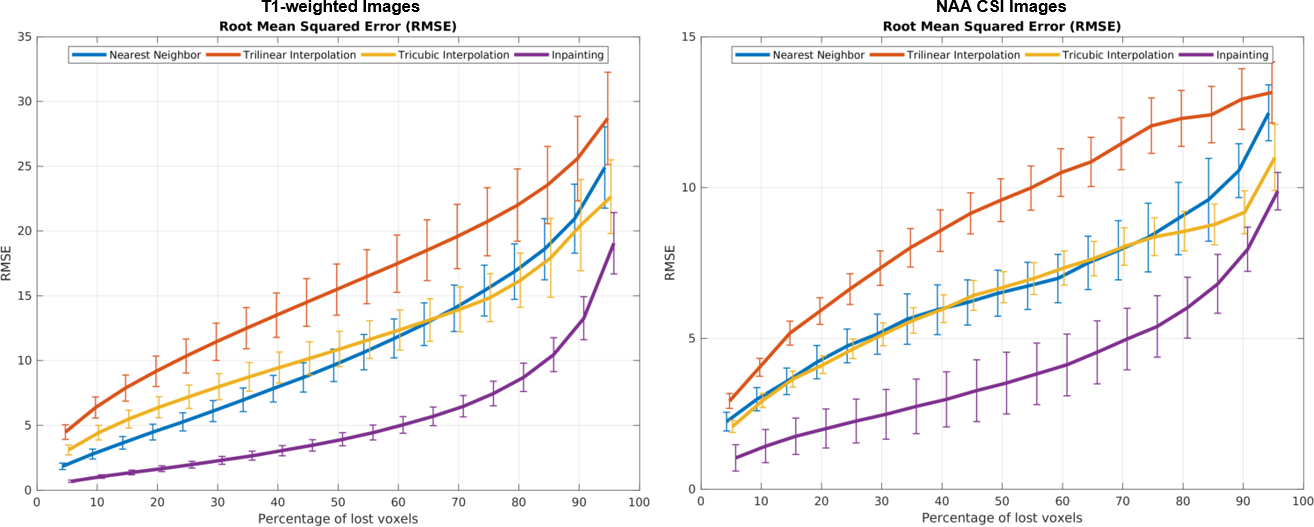
Figure 1 shows a visual example on how the different methods perform when interpolating random lost voxels from a T1-weighted image. Nearest neighbor interpolation introduces noise via quantization of the estimated values, and polynomial interpolation introduces error due to the fitting of the polynomial, while inpainting provides a closer result to the original image thanks to the inclusion of frequency information. Figure 2 shows the quantitative performance assessment of the different methods on high-resolution T1-weighted and NAA CSI images. The ANOVA analysis revealed a statistically significant effect of the method (T1:F3,51=1018.6,p<0.001; CSI:F3,51=298.5,p<0.001) and percentage of lost voxels (%loss; T1:F18,306=1122.6,p<0.001; CSI:F18,306=2179.1,p<0.001), as well as a statistically significant method*%loss interaction (T1:F54,918=123.3,p<0.001; CSI:F54,918=124.8,p<0.001), indicating that the advantage of inpainting, while generally observed across all %loss categories, becomes more evident with <85 or 90% loss.Discussion
Our findings demonstrate a drastic improvement in the restored data when using the inpainting approach, compared to other, classical interpolation methods (Fig 2). This improvement was seen for both T1 and CSI data, and was thus not varying across contrast type or voxel size. These methods will now need to be tested on images that are more likely to lead to voxel loss, such as metabolites presenting poorly-fitted voxels.Conclusion
Inpainting methods can help restoring poorly fitted CSI voxels with good accuracy. Among the various advantages of this methods is the possibility to minimize the number of voxels excluded from group analyses in standard space. To the best of our knowledge, this is the first work dealing with CSI interpolation/inpainting and these preliminary results could help to set the basis for future developments.Acknowledgements
Support: 1R21NS087472-01A1/1R01NS095937-01A1/W81XWH-14-1-0543/1R01NS094306-01A1 (MLL).References
1. Bertalmio M, Sapiro G, Caselles V, Ballester C. Image inpainting. In Proceedings of the 27th Annual Conference on Computer Graphics and Interactive Techniques, New Orleans, LA, USA – July 23-28, 2000, 2000;417-424. ACM Press/Addison-Wesley Publishing Co.
2. Andronesi OC, Gagoski BA, Sorensen AG. Neurologic 3D MR spectroscopic imaging with low-power adiabatic pulses and fast spiral acquisition. Radiology, 2012;262(2):647-661.
3. Provencher SW. Estimation of metabolite concentrations from localized in vivo proton NMR spectra. Magn Reson Med, 1993;30(6):672-679.
4. Garcia D. Robust smoothing of gridded data in one and higher dimensions with missing values. Comput Stat Data An, 2010;54(4):1167-1178.
Figures