2451
Bayesian Hierarchical Modelling for Analyzing Neuroimaging Results1Neuroscience and Mental Health, The Hospital For Sick Children, Toronto, ON, Canada, 2Medical Biophysics, University of Toronto, Toronto, ON, Canada
Synopsis
The most common analysis of structural brain MRIs involves massively univariate modelling. Such analyses separately approach different levels of resolution (whole brain, regional, and voxel) and do not provide an easy solution to understanding whether some areas of the brain are more or less affected than others. Here we explore applying hierarchical bayesian modelling to simultaneously analyze brain MRI studies at multiple levels of resolution while allowing for the explicit interrogation of whether brain areas are differentially affected. In addition, we show that hierarchical modelling provides improved parameter recapture, sign error rate, and model fit.
Intro
Massively univariate modelling of brain MRIs fits a linear model at
every brain structure, and then accounts for inflated false positives by
widening the confidence interval in order to correct for multiple
comparisons. Our proposed approach to bayesian hierarchical modelling of
anatomical brain MRIs also fits a linear model for every brain
structure, but constrains the fit by pooling the estimates for each
structure towards the fit for other structures, potentially further
elaborated by an explicit tree definining the relation between brain
structures1 (structure taxonomy). Partial-pooling, or shrinkage, thus replaces multiple
comparisons correction2. After fitting, the posterior can be interrogated
to both assess whether the model terms deviate from zero as well as
whether that deviation from zero is more or less in one structure than
another. The taxonomy describing the relation between structures also
allows for the identification of which level of resolution best
identifies effects.
We illustrate bayesian hierarchical modelling on a mouse MRI data-set
designed to assess sex differences in the brain. We compare standard
no-pooling (i.e. massively univariate) approaches with the
partial-pooling approach of bayesian hierarchical modelling. We show
that performance in key dimensions including parameter recapture and
sign error rates are enhanced by using these models.Methods
We test our models on volumes derived from automatically segmented T2 MRI scans of C57BL/6J mouse brains. Most are publicly available from the Ontario Brain Institute (https://www.braincode.ca/content/open-data-releases). We examined five studies with more than 20 male and 20 female mice to assess reliability of sex-difference estimation. Estimates were compared against the estimated sex-differences from all 587 C57BL/6J mice.
Models:
We examine two variants of the no-pooling model. Models shown in lme4 mixed-effects syntax where appropriate. All models are fit via rstan3 and rstanarm4.
- $$$y \sim sex$$$ fit at each structure.
- $$$y \sim sex + brain{\text -}volume$$$ at each structure.
We examine three bayesian hierarchical models:
- Flat hierarchy: $$$y \sim sex + (sex | structure) + (1 | mouse{\text -}id)$$$ across all structures.
- Parental hierarchy: $$$y \sim sex + (sex | structure) + (1 | super{\text -}structure) + (1 | mouse{\text -}id)$$$ across all structures. Our atlas is taxonomically organized such that each structure is a member of a larger super-structure.
- Effect diffusion tree: A model of our design that pools according to a full taxonomy of structures.
Metrics:
We compare the six models across the following dimensions:
- Parameter recapture. How well do the models applied to the 5 studies recover the parameters estimated from the full data set. These are evaluated by correlation and mean-squared-error.
- Type S error rate. Assesses the proportion of parameter estimates from the 5 studies that differ in sign from the estimates in the full data set.
- Model fit. How well do these models fit the observed data, evaluated with mean-squared-error.
- Predictive performance. How well do these generalize to unobserved data. Evaluated with pareto-smoothed importance-sampling approximate cross-validation5 (loo).
Results
In this work we show the advantage of bayesian hierarchical posterior
distributions (fig 1. left) for performing inference across structures.
We show how trivial it is to compare posterior estimates (fig 2.
right), respecting uncertainty without multiplicity correction.
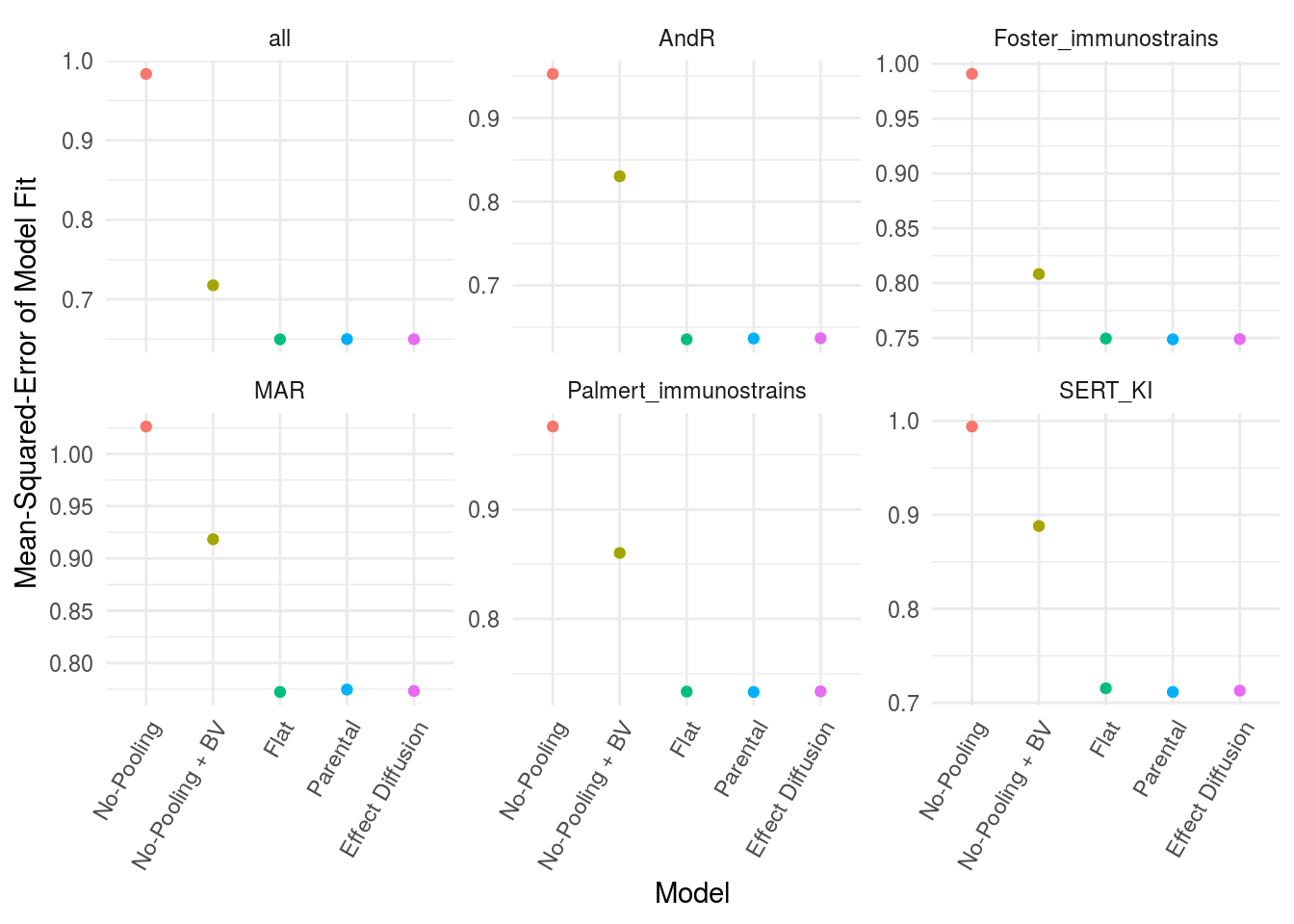
The results show that the bayesian models uniformly outperform the no-pooling models in terms of model fit (fig. 2). The information pooling of effects across structures, and intercepts across individuals substantially improves the mean-squared-error of model fit. Adding the whole brain volume as a covariate substantially remedies the performance deficit (especially fig. 2 panel “all”).
Gold-standard effect recovery for hierarchical models was superior to no-pooling (fig. 3), having higher correlations and lower mean-squared-error. With brain volume covaried, no-pooling performs comparably with the bayesian models, although the effect diffusion tree performs marginally better in both domains. The same holds for predictive performance (fig. 4) except, no-pooling with brain volume covaried performs better on one study and the full data-set. These two cases have larger sample sizes, potentially indicating reduced benefit from pooling with increased data.
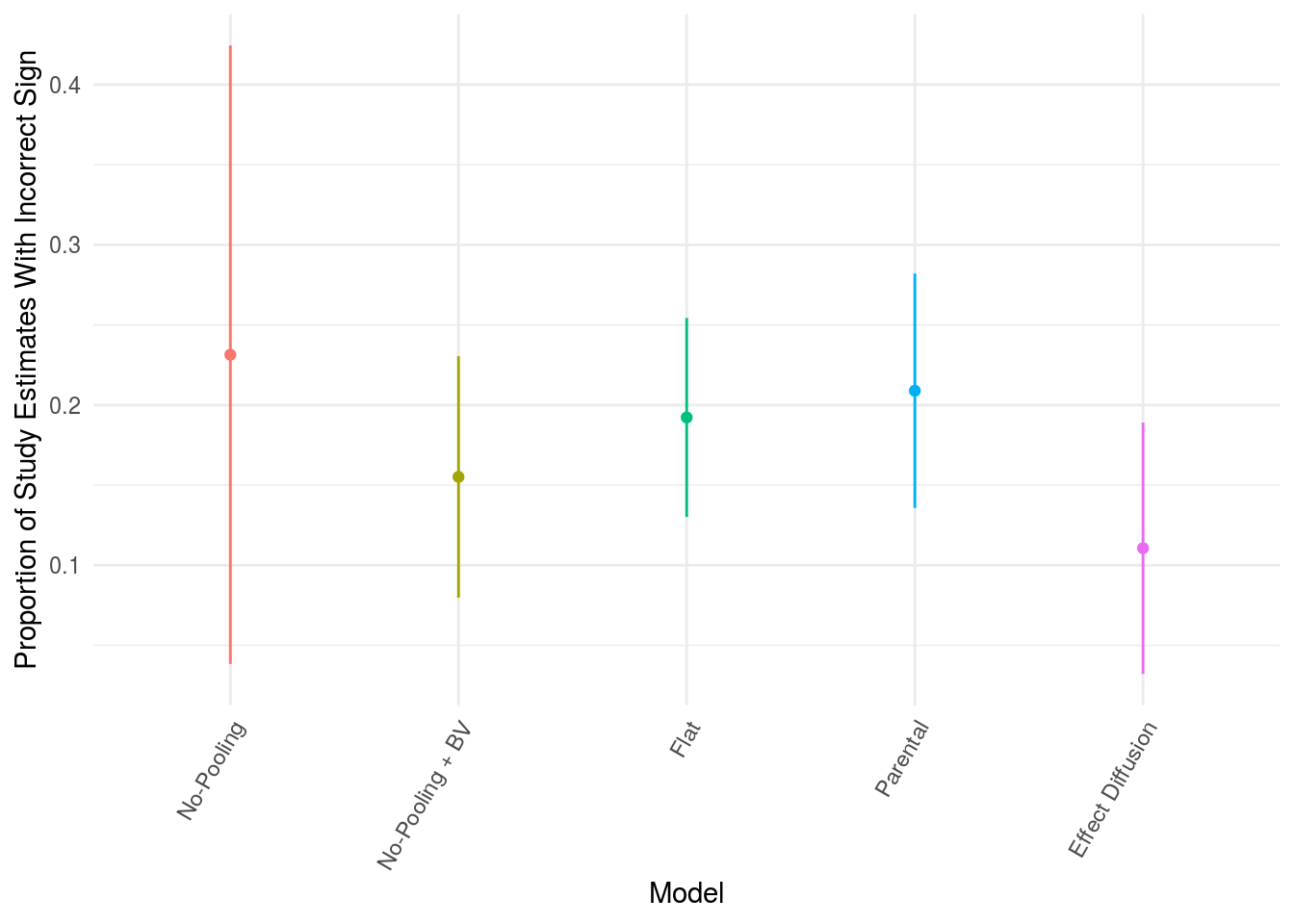
The bayesian models have marginally reduced sign error rates (fig. 5), relative to the no-pooling model, although comparable to the no-pooling with brain volume covaried. Again the effect diffusion tree performs best.
Conclusion
We show the utility of bayesian hierarchical modelling for enhancing model interrogation and improving parameter estimation. Bayesian hierachical models perform as well or better than standard no pooling models, and can be explored fully and simply without incurring multiplicity penalties.Acknowledgements
We would like to thank all members of the Mouse Imaging Centre for contributing data and thoughts throughout the development of this work, particularly Jacob Ellegood and Lily Qiu.References
1. Lein, Ed S, Michael J Hawrylycz, Nancy Ao, Mikael Ayres, Amy Bensinger, Amy Bernard, Andrew F Boe, et al. “Genome-Wide Atlas of Gene Expression in the Adult Mouse Brain.” (2007). Nature 445 (7124). Nature Publishing Group: 168.
2. Gelman, Andrew, Jennifer Hill, and Masanao Yajima. "Why we (usually) don't have to worry about multiple comparisons." Journal of Research on Educational Effectiveness 5.2 (2012): 189-211.
3. Stan Development Team. "Rstan: the R interface to Stan". (2018) R package version 2.18..
4. Goodrich B, Gabry J, Ali I & Brilleman S. (2018). rstanarm: Bayesian applied regression modeling via Stan. R package version 2.17.4. http://mc-stan.org/.
5. Vehtari A, Gelman A, Gabry J (2017). “Practical Bayesian model evaluation using leave-one-out cross-validation and WAIC.” Statistics and Computing, *27*, 1413-1432. doi: 10.1007/s11222-016-9696-4 (URL:http://doi.org/10.1007/s11222-016-9696-4).
Figures