2447
A Partial-Fourier Method Recovering Signal Loss from Off-resonance1Department of Electrical Engineering, Stanford University, Stanford, CA, United States, 2Department of Bioengineering, Stanford University, Stanford, CA, United States, 3Department of Radiology, Stanford University, Stanford, CA, United States
Synopsis
Functional MRI (fMRI) can have signal dropout due to off-resonance at susceptibility interfaces between air and tissue. Partial Fourier reconstruction is used for fMRI since it reduces scan time, however, existing partial Fourier reconstruction is vulnerable to off-resonance. In a previous study, we introduced a new partial Fourier reconstruction (even/odd (E/O)) and showed the new method was more robust to off-resonance compared to homodyne through simulation from fully sampled data. In this study, we acquired subsampled hypercapnia task fMRI data using both homodyne and E/O and showed there is less signal dropout and higher activation with E/O.
Introduction
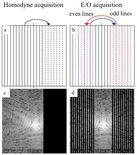
Since k-space has Hermitian symmetry for a real object, half of k-space data can be used to reconstruct MR images. Partial Fourier reconstruction reduces scan or readout time, therefore, it can be useful for functional MRI (fMRI) that requires long TE. One of the most widely used partial Fourier reconstruction methods is homodyne1. It requires one half k-space data and a few more lines at the center to overcome phase shifts. However, it is vulnerable to off-resonance, which is important for fMRI, because it loses most of the energy with a large amount of phase shift. As we introduced in a previous study2,3, even/odd (E/O) reconstruction method acquires even lines of one half, odd lines of the other half and additional full k-space line at the center (Fig. 1). In this study, we acquired breath-holding (BH) task fMRI using homodyne and E/O acquisitions and evaluated signal dropout and activation in terms of number of activated voxels in frontal brain area.Methods
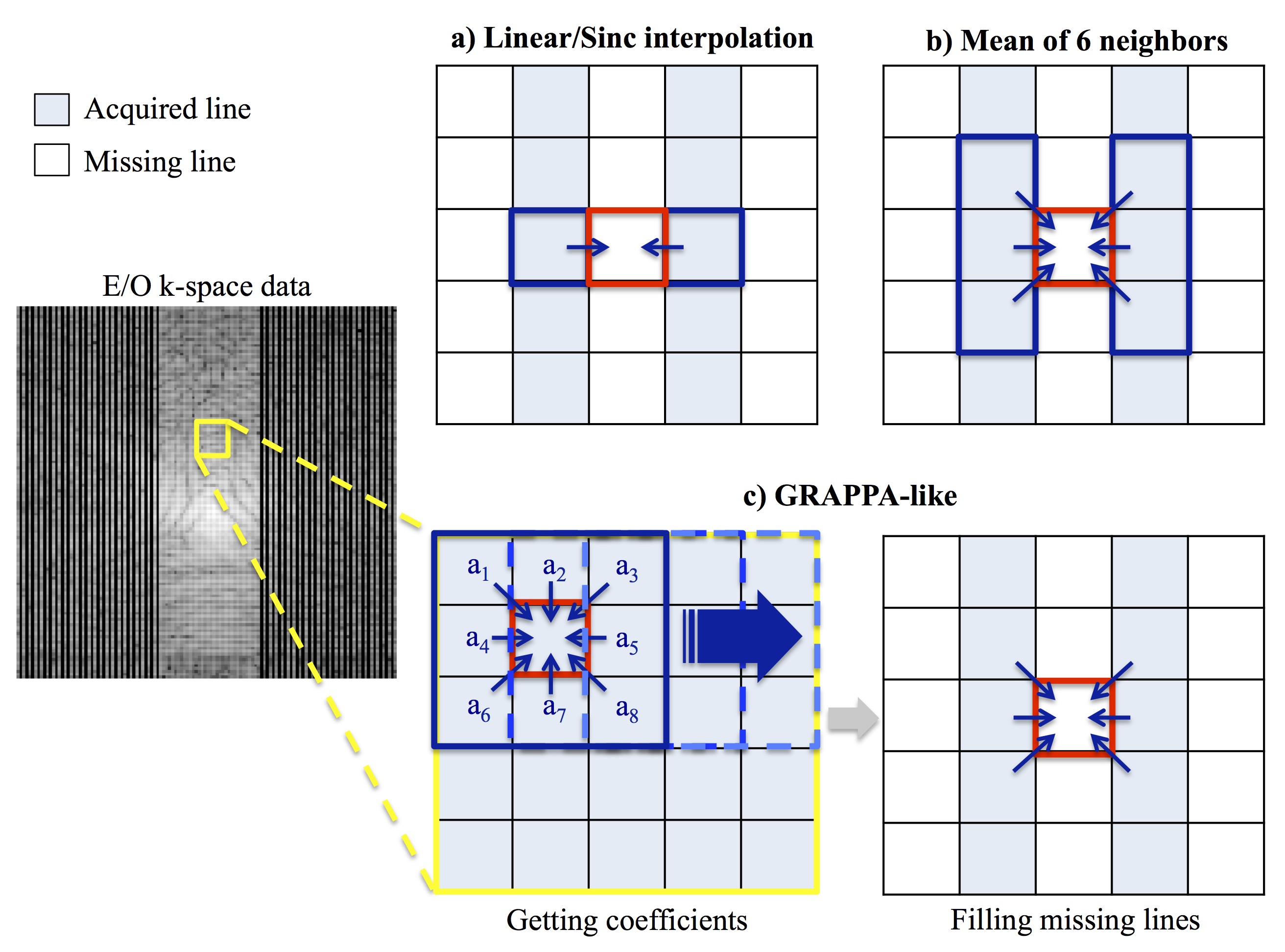
Data acquisition: With IRB approval, we scanned 10 human brains using a 2D EPI acquisition and a breath-holding (BH) task using homodyne and E/O sequence with TE/TR=30/2100 ms, 3.4 mm x 3.4 mm x 4 mm voxels, FOV=22 cm×22 cm, 30 slices, BW=500 Hz/pixel, flip angle=90 degrees, 146 timeframes and scan time=5min. We have acquired the same number of k-space lines for both methods (Fig. 1). Data analysis: For E/O, missing k-space data were filled with values that were created in four ways using neighboring voxels as we suggested in previous study3: The filling methods are 1) linear interpolation, 2) mean of six neighboring voxels, 3) sinc interpolation and 4) GRAPPA-like method (Fig. 2). Activation maps were created by correlating the data with sine/cosine functions that accounted for phase shifts from the hemodynamic response. We evaluated signal dropout from the reconstructed images and number of activated voxels from the activation maps. For the activation map, we set the ROIs to calculate the number of activated voxels (p<0.05) from frontal area of the brain. We normalized the number of activated voxels of E/O to that from homodyne for comparison.Results
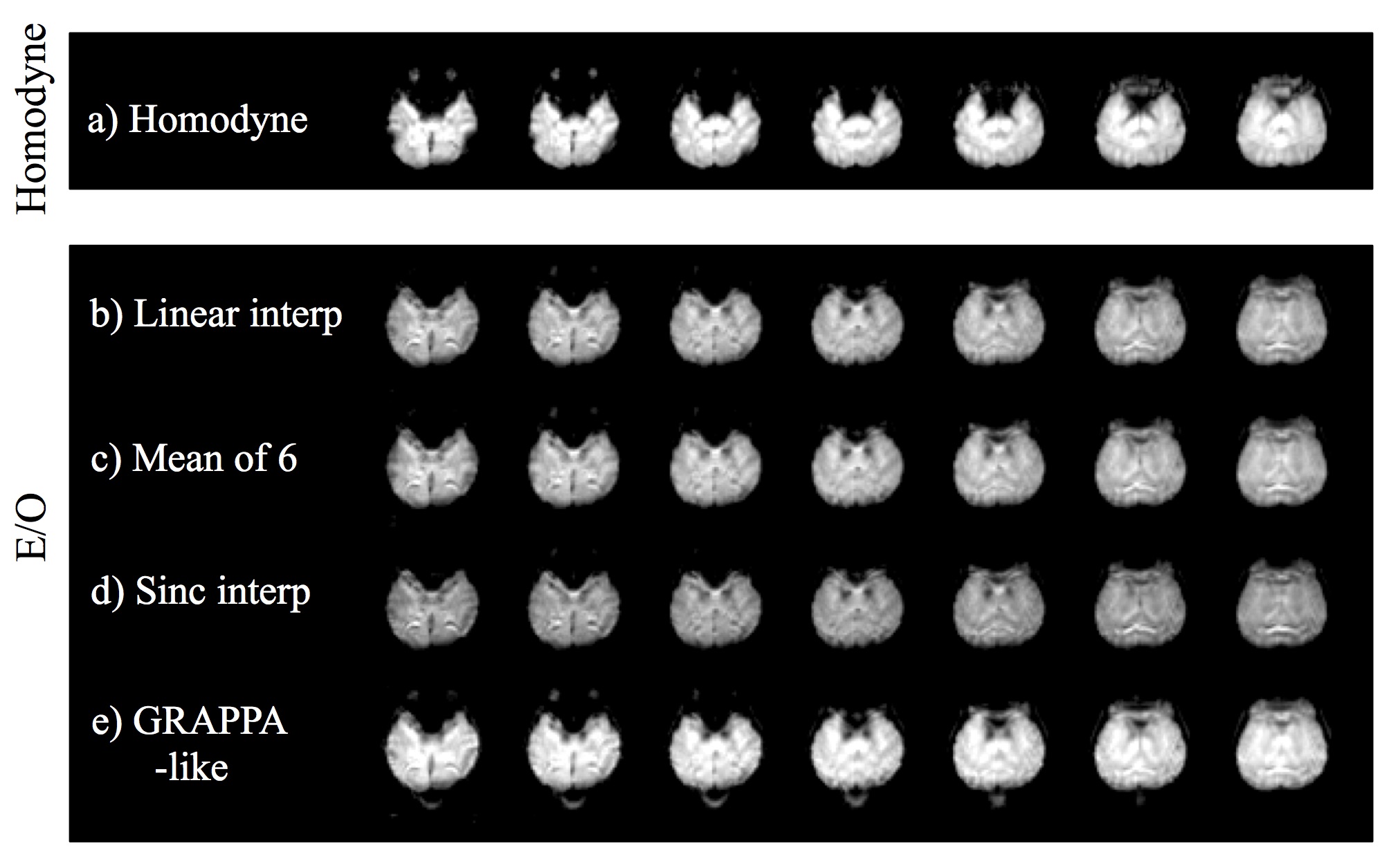
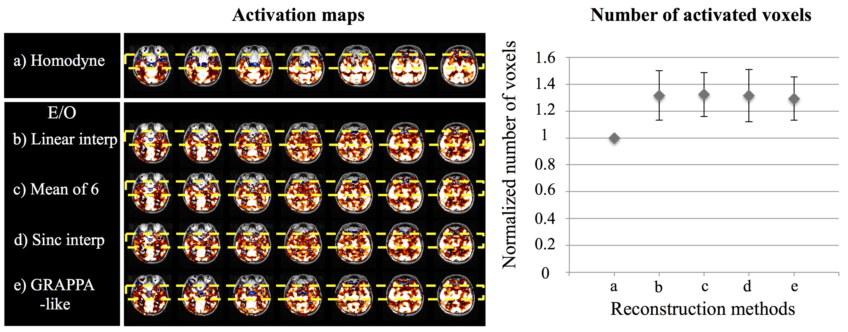
All the images from E/O with four methods for filling missing k-space lines (Fig. 3) showed less signal dropout in frontal lobe compared to those from homodyne even though the GRAPPA-like method showed more signal dropout in 12th -15th slices compared to the rest of the filling methods. Furthermore, all the E/O methods showed higher number of activated voxels compared to homodyne (Fig. 4). Average numbers of activated voxels of all the 10 subjects from each filling method show 31.6% higher (linear interpolation), 32.3% higher (mean of six neighbors), 31.5% higher (sinc interpolation) and 29.3% higher (GRAPPA-like) compared to those from homodyne and the differences are significant with p< 0.05.Discussion
We showed that E/O reconstruction is more robust to off-resonance compared to homodyne through simulations from fully sampled data in previous study. In this study, we acquired subsampled data using homodyne and E/O method and compared the reconstructed images and activation from hypercapnia task fMRI. E/O (with all the four filling methods) reconstructed successfully with less attenuation in air-tissue interfaces and showed higher activation in frontal brain area compared to homodyne.Acknowledgements
Funding for this work was provided by: NIH P41 EB015891References
1. Homodyne detection in magnetic resonance imaging. Noll D.C et al., Medical Imaging, IEEE Transactions on, 10(2):154-163,1991
2. Novel Half Fourier Reconstruction Recovering Signal Loss from Off-resonance. Lee S et al., Proceedings of the International Society for Magnetic Resonance in Medicine. 2016, p.1785
3. Strategies for Compensating for Missing k-space Data in a Novel Half-Fourier Reconstruction, Lee S et al., Proceedings of the International Society for Magnetic Resonance in Medicine. 2017, p.1512
Figures