2445

Joint Iterative Image Reconstruction and Field Map Estimation In Low Field MRI

Kirsten Koolstra¹, Merel de Leeuw den Bouter², Thomas O'Reilly¹, Peter Börnert^1,3, Rob Remis⁴, Martin van Gijzen², and Andrew Webb¹

¹C.J. Gorter Center for High Field MRI, Radiology, Leiden University Medical Center, Leiden, Netherlands, ²Institute of Applied Mathematics, Delft University of Technology, Delft, Netherlands, ³Philips Research Hamburg, Hamburg, Germany, ⁴Circuits and Systems, Delft University of Technology, Delft, Netherlands

Synopsis

Inaccuracies and temporal fluctuations in field map measurements form a major problem in image reconstruction for permanent magnet based low field MRI systems. These inaccuracies can potentially be corrected by using a joint image reconstruction and field map estimation algorithm. Simulation results show improved image quality when using a new updating scheme compared to standard iterative reconstructions.

Introduction

The design of low field portable MRI scanners is of great interest due to its potential clinical relevance in developing countries. Many of the systems have a highly inhomogeneous magnetic field, which can actually be used for spatial encoding and image formation^1–3. However, small inaccuracies in the field map, which can arise from temperature-induced changes or measurement errors, lead to image distortions. Therefore, an accurate field map is needed for each scan, but practically one cannot measure the field map for each scan. Here we propose an algorithm to estimate the field map in an iterative reconstruction, based on a general class of non-linear iterative least-squares estimation methods used, for example, in water/fat separation MRI⁴.

Methods

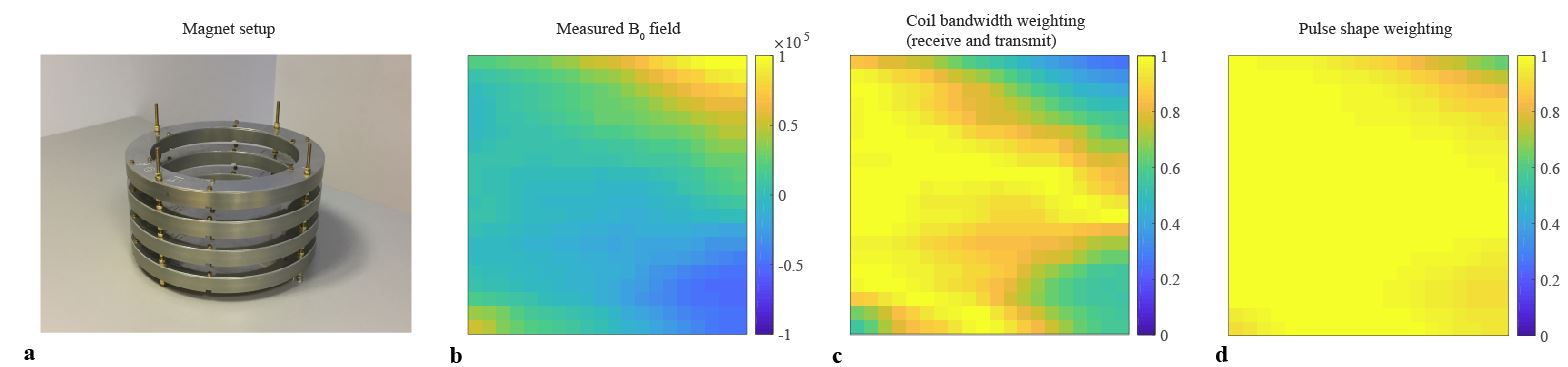
Experimental setup: A Halbach magnet was constructed, containing four rings each with 24 2.5×2.5×2.5 cm³ cubes of N-52 neodymium boron iron magnets (producing a 0.06T magnetic field at the center), with an internal ring of smaller magnets to produce a linear field gradient. The magnetic field was measured on a 5×7.5 mm² grid using a gaussmeter (Alphalab GM-2).

Simulation: A solenoid coil was modelled for RF transmission and reception. The sample was rotated 36 times with angular increments of $\theta =10$ °. For each rotation, a spin-echo sequence was simulated with RF pulse durations of 20 µs, and TE=5 ms; 512 data points and a dwell time of 2 µs. A signal model

$\textbf{S}_\theta=ETCR_\theta \textbf{m} \quad \text{(1)}$

was used with $\textbf{m}$ the unknown image (simulated as a Shepp Logan MATLAB phantom), $\textbf{S}_\theta$ the measured time-domain signal for rotation angle $\theta$ , $R_\theta$ the corresponding rotation matrix, $C$ a diagonal matrix with uniform spatial coil sensitivity weighted by the coil frequency profile (Q-factor of 13.8 based on an S₁₁ measurement) on the diagonal, $T$ a diagonal matrix including the pulse profile (simulated via the Bloch equations) and transmit bandwidth, $E$ the signal encoding matrix with elements $E_{pq}=e^{-2\pi iB_q t_p}$ , and $B_q$ the main field difference (with respect to the transmitter frequency) in Hz in pixel $q$ . White Gaussian noise was added to the signals such that the SNR was 10.

Image reconstruction: The image is reconstructed by solving the non-linear problem

$\hat{\textbf{m}}=\min \frac{\mu}{2}|| \sum_{\theta} \textbf{S}_\theta - ETCR_\theta \textbf{m} ||_2^2 + \frac{\lambda}{2} TV(\textbf{m}) \quad \text{(2)}$

where $TV$ is a total variation operator and $\mu$ and $\lambda$ regularization parameters. Substitution of the perturbations $\textbf{m}^R=\textbf{m}^R+\Delta \textbf{m}^R$ , $\textbf{m}^I=\textbf{m}^I+\Delta \textbf{m}^I$ and $\textbf{B}=\textbf{B}+\Delta \textbf{B}$ in Eq. (1) gives a system for the error terms:

$\sum_\theta A_\theta^H \left[ \begin{matrix} \textbf{S}_\theta^R -\textbf{a}_1 \\ \textbf{S}_\theta^I - \textbf{a}_2 \end{matrix} \right] = \sum_\theta A_\theta^H A_\theta \left[ \begin{matrix} \Delta \textbf{m}^R \\ \Delta \textbf{m}^I \\ \Delta \textbf{B} \end{matrix} \right] \quad \text{(3)}$

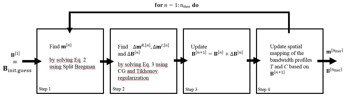
$\textbf{S}_\theta^R/\textbf{S}_\theta^I$ are the real/imaginary parts of the sampled time signal at rotation angle $\theta$ . $A_\theta$ describes the linearized data model for the error terms and $\textbf{a}_1/\textbf{a}_2$ describe the simulated time domain signal based on the estimated image $\textbf{m}$ . The final image is reconstructed by the algorithm shown in Figure 1.

Results

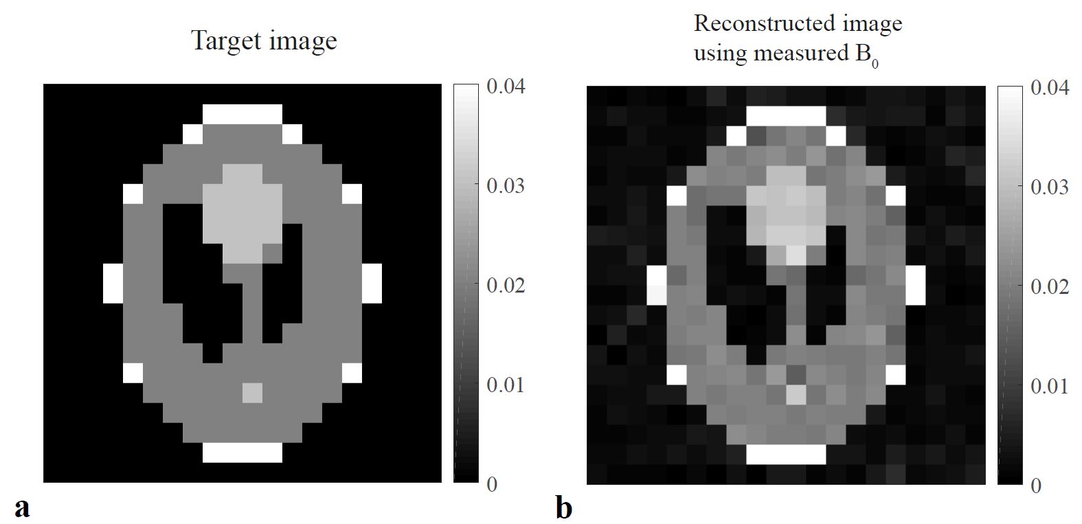
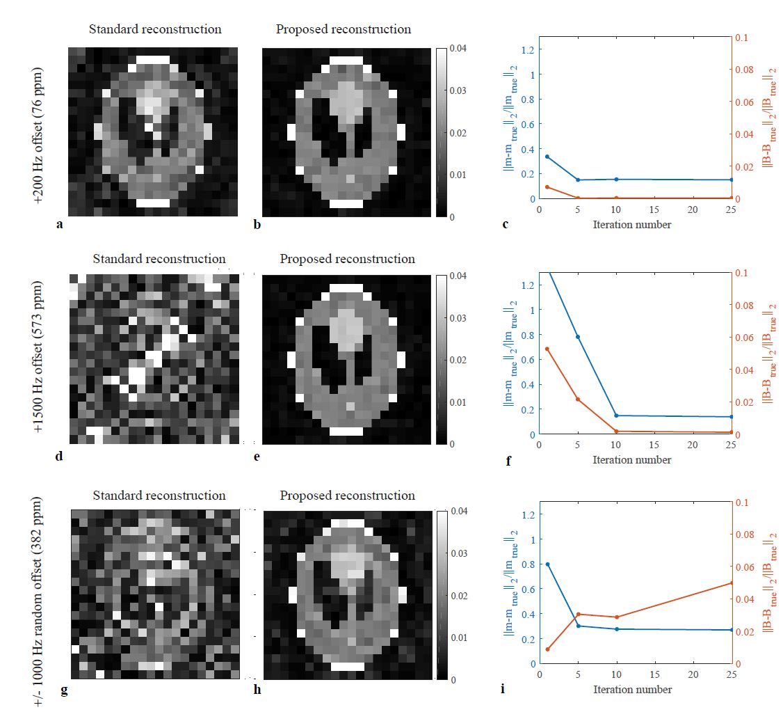
Figure 2 shows the magnet, the measured field map, the frequency profile of the Tx/Rx coil, and the weighting introduced by the pulse shape. The simulated phantom is shown in Figure 3 discretized at 5 mm resolution together with the reconstructed image using the measured field as the encoding function. Figure 4 shows how the image quality degrades if the field map is shifted by (a) 200 Hz and (d) 1500 Hz for each pixel in the reconstruction, corresponding to small uniform magnet/system temperature changes of 0.1°C and 0.5°C, respectively. Figures 4b,e show the reconstructed images after 25 iterations of the proposed scheme. The relative errors of the field and the image decrease with the number of iterations, as shown in Figures 4c,f. Figures 4g-i show results for a spatially random error in the field of between -1000 and +1000 Hz.

Discussion

Simulation results showed that distortions in the field map can be corrected by simultaneously estimating the field map and image in the reconstruction process. The quality of the reconstructed images after 25 iterations is comparable to that of the images reconstructed with the true field map. For very large field distortions a second-order error model could improve the reconstruction. The field inhomogeneity spatially encodes the time-domain signals, but the encoding power is relatively weak, resulting in an ill-posed minimization problem: further magnet optimization could increase the reconstruction performance in these low-encoding regions. Future work should investigate whether this algorithm can be extended to correct for continuous field drifts during the measurement.

Conclusion

The joint field map estimation and image reconstruction algorithm is able to improve the image quality in low field MRI in the presence of uncertainties in the field map.

Acknowledgements

This project was funded by the European Research Council Advanced Grant 670629 NOMA MRI.

References

1. Cooley C, Stockmann J, Armstrong B, et al. 2D Imaging in a Lightweight Portable MRI Scanner without Gradient Coils. Magnetic Resonance in Medicine. 2015;72(3):1–15.

2. Ren Z, Obruchkov S, Lu D, et al. A Low-field Portable Magnetic Resonance Imaging System for Head Imaging. Progress in Electromagnetics Research Symposium. 2017:3042–3044.

3. Cooley C, Haskell M, Cauley S, et al. Design of Sparse Halbach Magnet Arrays for Portable MRI Using a Genetic Algorithm. IEEE Transactions on Magnetics. 2017;54(1):1–12.

4. Reeder S, Wen Z, Yu H, et al. Multicoil Dixon Chemical Species Separation With an Iterative Least-Squares Estimation Method. Magnetic Resonance in Medicine. 2004;51(1):35–45.

Figures

Figure 1. Image reconstruction and field estimation algorithm. In step 1 an estimate of the image is found by solving problem (2) using Split Bregman. 6 outer iterations and 1 inner iteration were used for each iteration of the proposed scheme. Error estimates are found in step 2 by solving Eq. (3) using CG and Tikhonov regularization in which the finite difference regularization matrix enforces smoothness of the field error terms. Finally, the field map is updated using the estimates of the error terms and the transmit and receive maps are updated accordingly.

Figure 2. (a) Photograph of four ring Halbach magnet. (b) Difference field map in Hz (with respect to the transmitter frequency) measured with a Hall probe with a resolution of 5×7.5 mm² within a 10×10 cm² FOV, and rescaled to the desired reconstruction resolution using interpolation. (c) The bandwidth of the transmit/receive coil (Q-factor of 13.8) was normalized and spatially mapped to the measured field map. (d) The effect of the pulse shape and length on the flip angle distribution was taken into account by spatially mapping the normalized frequency profile of the pulse to the measured field map.

Figure 3. Image Reconstruction. (a) Simulated head (Shepp Logan MATLAB phantom) that was used to generate time-domain signals with an SNR of 10, using the measured field map in the signal model. (b) An image was reconstructed from these signals using the Split Bregman algorithm with total variation regularization. The desired resolution of 5 mm is obtained with a 20×20 reconstruction matrix. Regularization parameters were empirically defined and set to μ=2·10^-4, λ=200.

Figure 4. Joint image reconstruction and field map estimation. The quality of the image degrades when the field map contains a frequency shift of (a) 200 Hz (76 ppm) and (d) 1500 Hz (573 ppm) for each pixel, and random measurement errors between (g) -1000 and +1000 Hz (±382 ppm). (b,e,h) After 25 iterations of the joint reconstruction scheme the quality is much closer to that of the target image in Figure 3a. Small errors are still present in (h), for which the smoothness assumption of the field error does not hold. (c,f,i) The relative error decreases with the iteration number.

Proc. Intl. Soc. Mag. Reson. Med. 27 (2019)

2445