2427
Spatial-Temporal Super-Resolution Technique on Complex-Valued T2*-Weighted Dynamic MRI1Biomedical Engineering, University of Arizona, BIO5 institute, Tucson, AZ, United States
Synopsis
We present an approach for improving spatial and temporal resolution of complex-valued T2*-weighted dynamic MRI. Compared with traditional magnitude-valued spatial super-resolution method, our technique can better recover signal loss caused by the susceptibility dephasing effect. We propose that phase information can be utilized in spatial super-resolution to reduce the dephasing artifact. The feasibility of temporal super-resolution using complex-valued data is also separately evaluated for time-signal variation recovery. One limitation of our temporal super-resolution approach, which will be addressed in our future work, is the presence of leakage artifacts in the recovered time-signal due to linear interpolation bias.
Introduction
High spatial and temporal resolution are necessary to maximize the sensitivity and specificity of T2*-weighted dynamic MRI which can be applied to dynamic susceptibility contrast and functional MRI for clinical and research applications but are challenging to obtain due to the restriction of image acquisition time. Increased spatial resolution in the slice-selection direction necessitates the acquisition of thin slices which suffer from low SNR. Increased temporal resolution is constrained by TE (~T2*) required for optimal contrast and by T1 saturation effects which also reduce SNR1. One approach to resolving these challenges is to use super-resolution2 to reconstruct high resolution images using sub-voxel spatially-shifted low resolution images3, 4. A previous study5 has shown the feasibility of using super-resolution in MRI image reconstruction for through-plane resolution improvement. Peeters et al. have further shown the effectiveness of super-resolution for fMRI data acquired with thicker slices on 1.5T scanner6. Multiband-based super-resolution approaches like SLIDER-SMS7, 8 have recently been proposed to make high spatial and temporal super-resolution of fMRI feasible for clinical 3T and 7T scanners. However, T2*-weighted dynamic MRI is known to suffer from dephasing when thicker slices are acquired. This is a limitation of spatial super-resolution approaches on dynamic MRI that needs to be addressed. In this project, we compared the degree of signal-loss recovery due to the dephasing effect for T2*-weighted dynamic MRI between using complex-valued data and magnitude-valued data.Methods
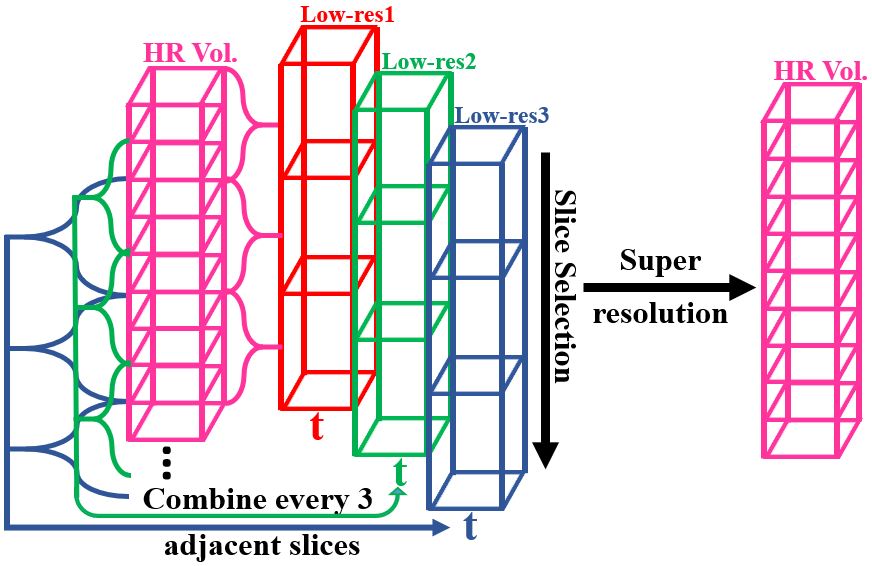
1). Complex-valued spatial super-resolution: The general process is shown in Fig. 14. Complex-valued T2*-weighted high-resolution dynamic MRI data (human brain and mouse heart) was acquired using gradient echo sequence. Three sets of sub-voxel shifted low resolution images were then created by combining every three adjacent slices of the complex-valued high resolution image, assuming no time-signal variation. The smoothed complex-valued high-resolution image and the mean of the interpolated image from the magnitudes of the three sets of low-resolution images were used as regularization reference images for complex-valued super-resolution and magnitude-valued super-resolution, respectively, with the regularization parameter λ =0.2 (Tikhonov regularization), which was determined experimentally to be optimal for both approaches. The reconstruction results generated from complex-valued super-resolution and magnitude-valued super-resolution were evaluated and compared in terms of recovering signal loss due to susceptibility dephasing effect.
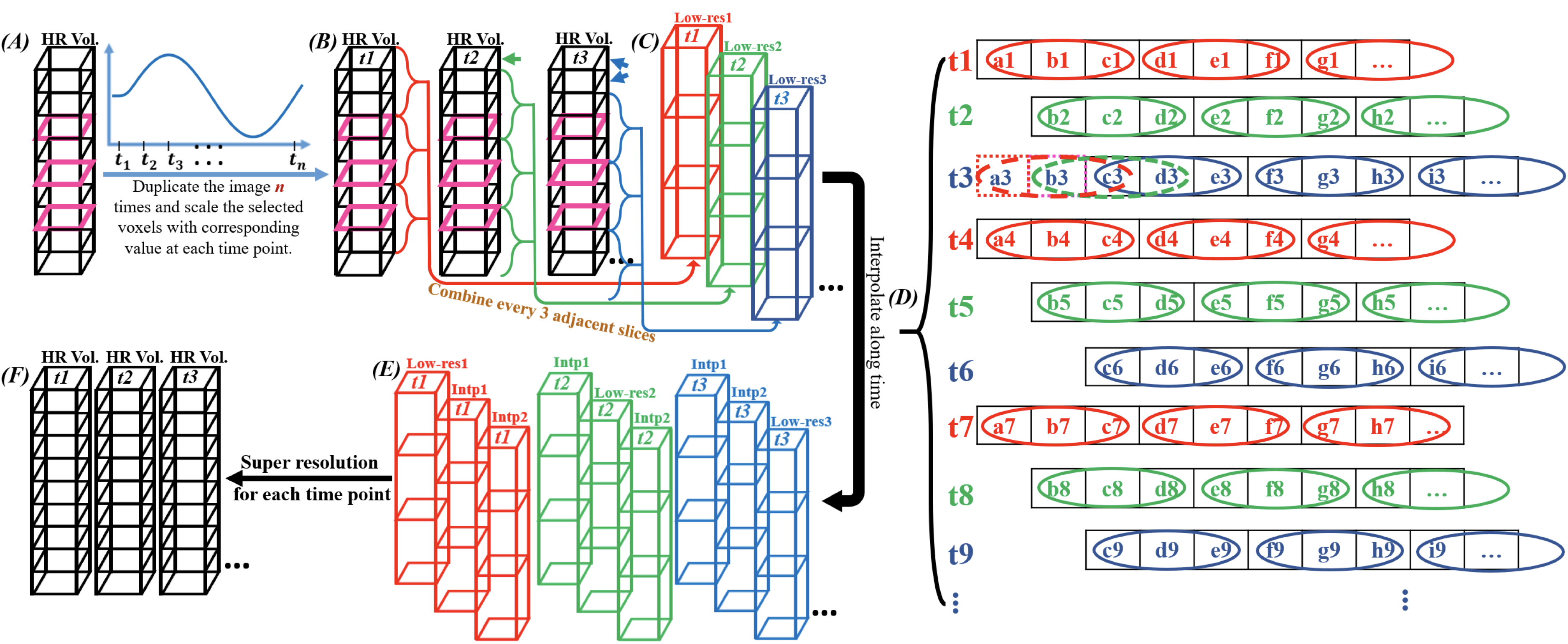
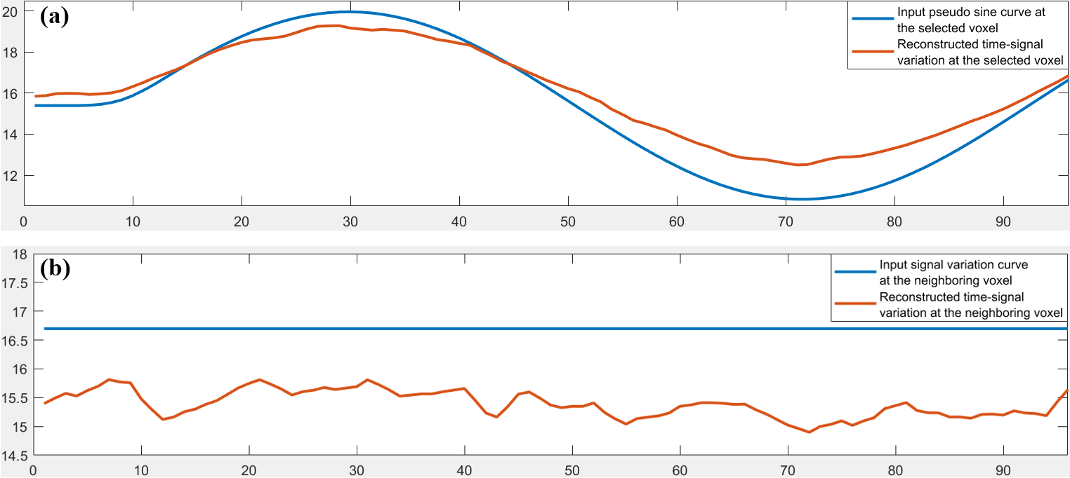
2). Complex-valued temporal super-resolution: The general process is illustrated in Fig. 2. A pseudo smooth sine curve with 101-time points and amplitude ranging from 0.7 to 1.3 was used to represent the relative dynamic change of signal intensity (Fig. 2(A)). The signal intensities within several selected voxels in the complex-valued high-resolution mouse heart MRI data were weighted by the pseudo sine curve, whereas the rest voxels were weighted by a constant value. The complex-valued sub-voxel shifted low-resolution images relative to different time points were then formed by summing every three adjacent voxels at each time point (Fig. 2(B and C), the arrows in (B) represent sub-voxel shifts), Gaussian noise was added afterwards. The other two sub-voxel shifted low-resolution images at each time point were generated through 1D linear interpolation along the time dimension (Fig. 2(D)). The letters a1, b1, c1, etc. represent signal intensity at each voxel along the slice-selection direction; c3 d3 e3 were combined at time point t3, and a3 b3 c3 and b3 c3 d3 were created using the interpolation between time points t1 and t4, and t2 and t5, respectively. The reconstructed signal was compared with the input sine curve.
Results
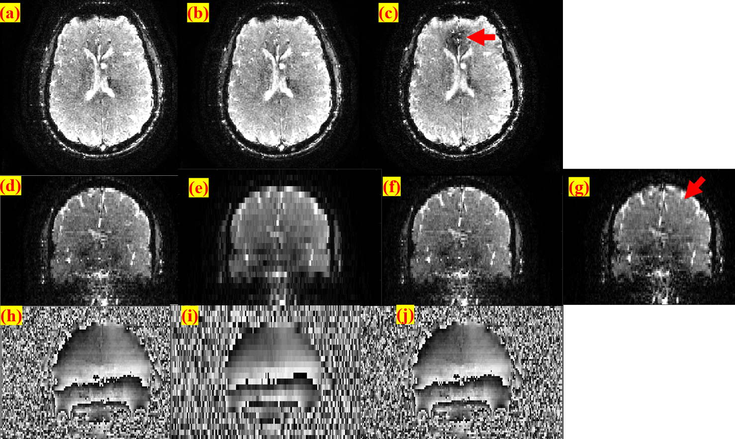
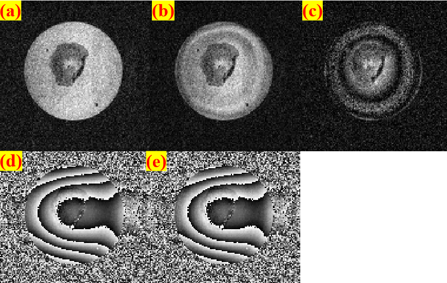
The complex-valued super-resolution has better performance than the magnitude-valued super-resolution in recovering the signal loss due to dephasing effect in both human brain data and muse heart data (Fig.3(a)~(c) and Fig.4). As can be seen from Fig.3(d)~(g), complex-valued super-resolution has better improvement on resolution than magnitude-valued super-resolution. The time variation of the original sine input can also be recovered accurately at the voxels weighted by the input sine signal (Fig.5(a)). However, the neighboring voxels that do not possess any signal-time variations show spurious signal changes with time after temporal super-resolution because of signal leakage caused by the linear interpolation (Fig.5(b)). The magnitude of the signal fluctuation though is relatively small.Discussion
Fig.3 and Fig.4 show the improved effectiveness of complex-valued super-resolution (Fig.3(b) and Fig.4(b)) in signal recovery over magnitude-value super-resolution, which still presents dephasing artifact (Fig.3(c) and Fig.4(c)). In complex-valued temporal super-resolution, several leading and trailing time points were discarded since the boundary of the time points usually involves extrapolation which would be inaccurate. This agrees with the practical dynamic MRI acquisition where the initial volumes obtained prior to scanner equilibrium are discarded. The time-signal leakage into neighboring voxels, as shown in Fig.5(b), is due to imperfections with the super-resolution linear interpolation. Future effort will focus on improving our approach to minimize this artifact.Acknowledgements
No acknowledgement found.References
1 Glover GH. Overview of Functional Magnetic Resonance Imaging. Neurosurg. Clin. N. Am. 2011; 22(2): 133–139.
2 Tsai, R.Y.; Huang, T.S. Multiframe image restoration and registration. In Advances in Computer Vision and Image Processing; JAI Press: Greenwich, CT, USA, 1984; Volume 1, pp. 317–339.
3 Li L, Wang W, Luo H, Ying S. Super-Resolution Reconstruction of High-Resolution Satellite ZY-3 TLC Images. Sensors 2017; 17(5).
4 Van Reeth E, Tham IWK, Tan CH, Poh CL. Super-resolution in magnetic resonance imaging: A review. Concepts Magn. Reson. Part A 2012; 40A(6): 306–325.
5 Greenspan H, Oz G, Kiryati N, Peled S. MRI inter-slice reconstruction using super-resolution. Magn. Reson. Imaging 2002; 20(5): 437–446.
6 Peeters RR, Kornprobst P, Nikolova M, et al. The use of super-resolution techniques to reduce slice thickness in functional MRI. Int. J. Imaging Syst. Technol. 2004; 14(3): 131–138.
7 Setsompop K, Fan Q, Stockmann J, et al. High-resolution in vivo diffusion imaging of the human brain with generalized slice dithered enhanced resolution: Simultaneous multislice (gSlider-SMS). Magn. Reson. Med. 2018; 79(1): 141–151.
8 Vu AT, Beckett A, Setsompop K, Feinberg DA. Evaluation of SLIce Dithered Enhanced Resolution Simultaneous MultiSlice (SLIDER-SMS) for human fMRI. NeuroImage 2018; 164: 164–171.
Figures