2421
A Neural Network for Rapid Generation of Cardiac MR Fingerprinting Dictionaries with Arbitrary Heart Rhythms1Biomedical Engineering, Case Western Reserve University, Cleveland, OH, United States, 2Computer Science, Johns Hopkins University, Baltimore, MD, United States, 3Radiology, University Hospitals, Cleveland, OH, United States
Synopsis
Cardiac MR Fingerprinting with ECG gating typically requires that a new Bloch equation simulation
Introduction
Cardiac MR Fingerprinting (cMRF) enables the simultaneous quantification of T1, T2, and M0.1,2 However, since the scan is ECG-gated, the cardiac rhythm must be incorporated in the dictionary simulation to obtain accurate measurements. This may impede clinical translation, especially if computationally expensive corrections are modeled, such as slice profile or preparation pulse efficiency.3 Inspired by recent work combining machine learning and MRF,4–6 this study uses a neural network to rapidly generate cMRF dictionaries for arbitrary heart rhythms.Methods
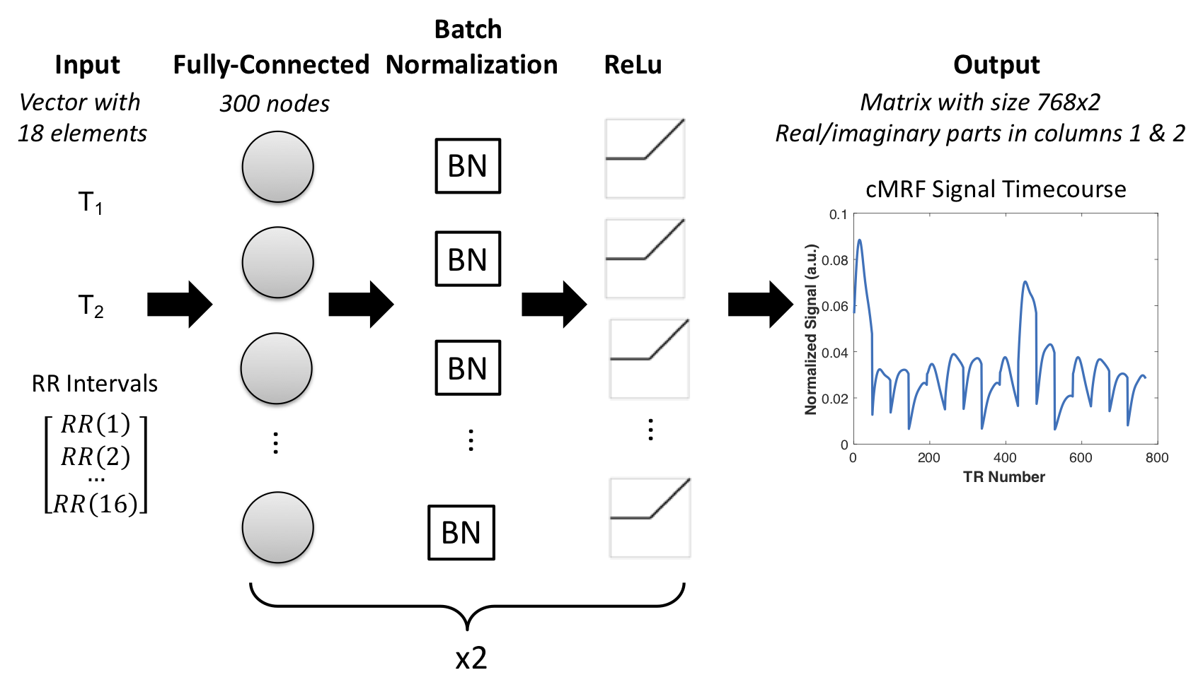
A 16-heartbeat cMRF sequence was used as described previously.2 Figure 1 shows a diagram of the neural network, which takes as inputs T1, T2, and the RR interval times between heartbeats, and outputs a complex-valued signal evolution. The network was trained using 510 simulated cardiac rhythms with average heart rates 40-120bpm (5bpm step size). For each average heart rate, 30 cardiac rhythms were simulated by adding random Gaussian noise with standard deviation 0-50% of the mean RR interval. The Bloch equations with corrections for slice profile and preparation pulse efficiency3 were used to simulate 4392 signal timecourses for each rhythm with T1 50-3000ms and T2 2-600ms. The total number of cMRF timecourses available for training was 510(cardiac rhythms) x 4392(parameter combinations) = 2.2x10⁶. Training was performed in MATLAB using an ADAM optimizer, mini-batch size 256, 100 epochs, and learning rate 0.01.
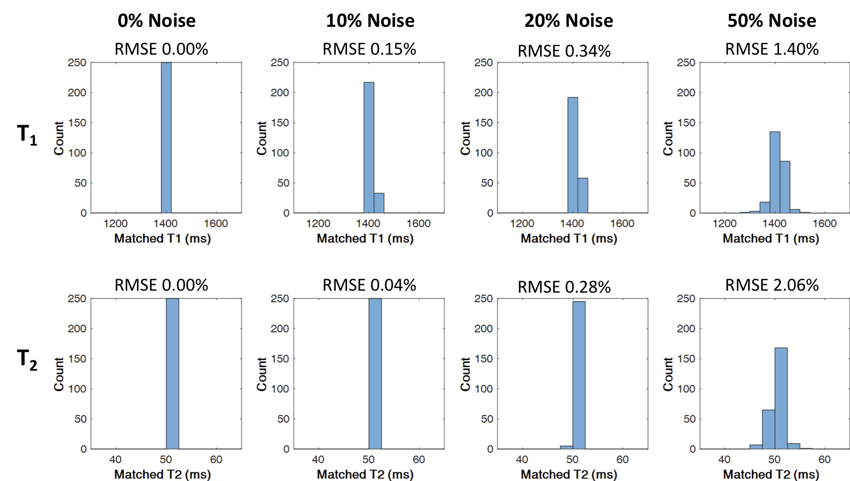
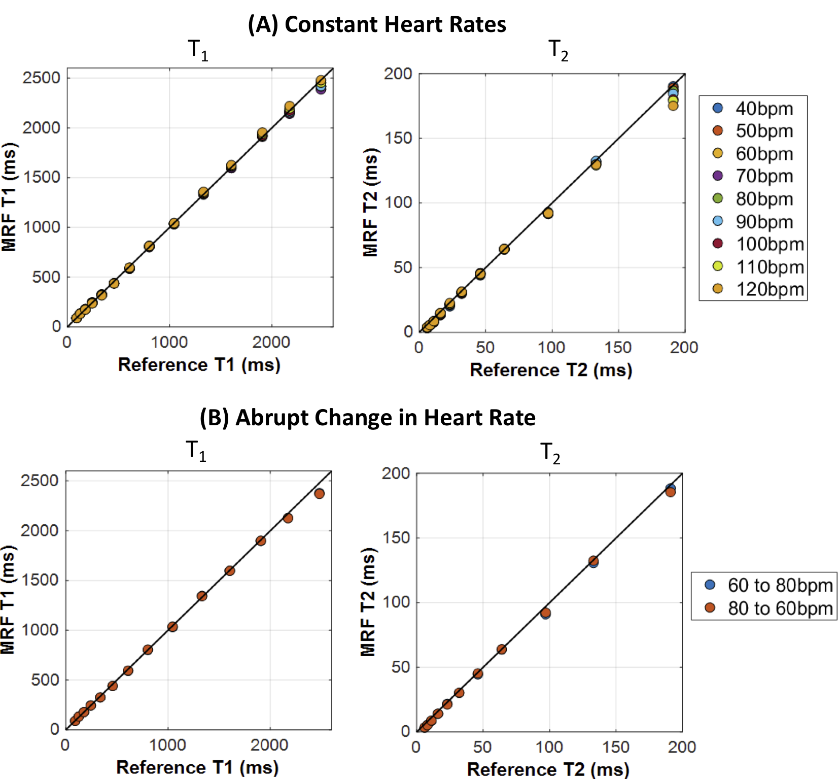
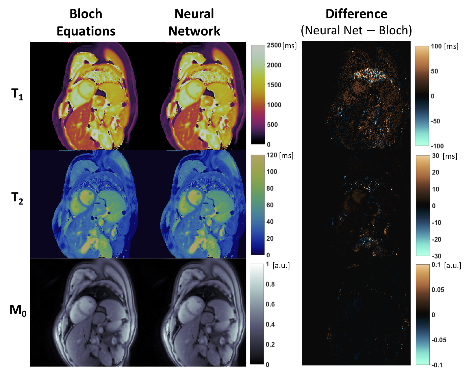
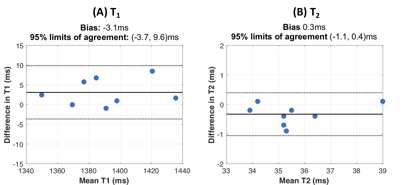
Monte Carlo simulations were conducted to test performance under variable heart rate conditions. Reference signals representative of myocardium (T1=1400ms, T2=50ms) were simulated for cardiac rhythms having an average 63bpm, chosen because this heart rate was not present during training, and matched to a dictionary produced by the network. Random Gaussian noise with standard deviations of 0%,10%, 20%, and 50% of the mean RR interval was added to the cardiac cycle. The simulation was repeated 250 times for each noise level, and errors were quantified using normalized RMSE. Next, the T2 array of the ISMRM/NIST system phantom7 was scanned at 3T (Siemens Skyra) using an 18-channel head coil array. Data were acquired using a variable density spiral8 with golden angle rotation,9 192x192 matrix, 300mm2 FoV, and 8mm slice thickness. Data were collected with constant heart rates of 40-120bpm (step size 10bpm) simulated at the scanner. Two scans were acquired where the heart rate changed abruptly from 60 to 80bpm (and 80 to 60bpm) after 8 heartbeats. Dictionaries with identical T1 and T2 discretization were generated using the Bloch equations and the neural network. Undersampled images were gridded using the NUFFT10 and matched to each dictionary using the inner product to generate parameter maps. A similar experiment was conducted using in vivo data acquired in 8 volunteers in an IRB-approved, HIPAA-compliant study after obtaining written informed consent. T1 and T2 values were measured in the septal wall, and the agreement between Bloch equation vs neural network approaches was assessed using a Bland-Altman analysis.11
Results
After training for 4 hours, the time to generate a dictionary with 26,680 entries was 0.8s (neural network) vs 158s (Bloch equations using parallelized MATLAB Mex code). Figure 2 shows the Monte Carlo simulation results. The neural network estimates under constant heart rate conditions (0% noise) are nearly perfect. Errors increase as heart rates become more variable but remain small (RMSE<1%) up to a noise level of 20%. Figure 3 shows results from the phantom scan. The neural network produced accurate T1 and T2 measurements for constant heart rates between 40-120bpm, although high T2 values (near 200ms) were slightly underestimated at high heart rates. Accurate measurements were also obtained when the heart rate changed abruptly halfway during the scan. Representative in vivo maps are shown in Figure 4. Excellent agreement between the Bloch equation and neural network approaches was observed, as corroborated by the Bland-Altman plots in Figure 5.Discussion
This study demonstrates that a neural network can generate cMRF timecourses for arbitrary cardiac rhythms. Once trained, the network can output a dictionary over 100 times faster than a Bloch equation simulation with parallelized Mex code. Eliminating the need perform a Bloch equation simulation after every scan could accelerate online reconstructions and facilitate clinical translation of cMRF. Corrections for system imperfections, which may be time-consuming to model, can be included upfront in the network training. Future work will investigate new network architectures and the use of actual, rather than simulated, cardiac rhythms for training to improve performance.Conclusion
A neural network is introduced for rapidly generating cMRF dictionaries for arbitrary heart rhythms, eliminating the need to perform a Bloch equation simulation after every cMRF scan.Acknowledgements
NIH R01HL094557, R01DK098503, R01EB016728; NSF CBET 1553441, Siemens Healthineers (Erlangen, Germany)References
- Ma D, Gulani V, Seiberlich N, et al. Magnetic resonance fingerprinting. Nature. 2013;495(7440):187-192.
- Hamilton JI, Jiang Y, Chen Y, et al. MR fingerprinting for rapid quantification of myocardial T1, T2, and proton spin density. Magn Reson Med. 2017;77:1446-1458.
- Hamilton JI, Jiang Y, Ma D, et al. Investigating and reducing the effects of confounding factors for robust T1 and T2 mapping with cardiac MR fingerprinting. Magn Reson Imaging. 2018;53:40-51.
- Cohen O, Zhu B, Rosen MS. MR fingerprinting Deep RecOnstruction NEtwork (DRONE). Magn Reson Med. 2018;80(3):885-894.
- Hoppe E, Körzdörfer G, Würfl T, et al. Deep Learning for Magnetic Resonance Fingerprinting: A New Approach for Predicting Quantitative Parameter Values from Time Series. Stud Health Technol Inform. 2017;243:202-206.
- Yang M, Jiang Y, Ma D, Mehta BB, Griswold MA. Game of Learning Bloch Equation Simulations for MR Fingerprinting. Proc. ISMRM 2018; #673.
- Russek SE, Boss M, Jackson EF, et al. Characterization of NIST/ISMRM MRI System Phantom. Proc. ISMRM 2012; #2456.
- Hargreaves B. Variable-Density Spiral Design Functions. http://mrsrl.stanford.edu/~brian/vdspiral/. Published 2005. Accessed June 1, 2017.
- Winkelmann S, Schaeffter T, Koehler T, Eggers H, Doessel O. An optimal radial profile order based on the Golden Ratio for time-resolved MRI. IEEE Trans Med Imaging. 2007;26(1):68-76.
- Fessler J, Sutton B. Nonuniform fast Fourier transforms using min-max interpolation. IEEE Trans Signal Process. 2003;51(2):560-574.
- Bland JM, Altman DG. Statistical methods for assessing agreement between two methods of clinical measurement. Lancet. 1986;1(8476):307-310.
Figures