2419
Rapid prOtotyping of 2D non-Cartesian K-space trajEcTories (ROCKET)1Dayananda Sagar Institution, Bangalore, India, 2Columbia Magnetic Resonance Research Centre, Columbia University, New York, NY, United States, 3Wipro GE Healthcare, Bangalore, India
Synopsis
Rapid prOtotyping of 2D non-CartesIan K-space trajEcTories (ROCKET) aims to aid researchers interested in rapid development and testing of new MR methods starting from pulse sequence design to image analysis. This was achieved by utilizing Pulseq for pulse sequence design and graphical programming interface for image reconstruction and analysis. ROCKET was demonstrated on two non-Cartesian k-space trajectories – FID based radial and spiral. Each trajectory was tailored into three different trajectories based on rotating angle – standard, golden angle and tiny golden angle. All studies were performed on Siemens scanner demonstrated on in-vitro phantom and in-vivo healthy brain acquisitions and SNRs were computed.
Introduction
Cartesian trajectory based acquisition is routinely used in clinical MR studies. However, it takes long time for acquisition which is the major limiting factor. Dynamic scans such as cardiac MRI and dynamic contrast enhanced MRI demand fast acquisition, which can be achieved by using non-Cartesian based acquisition. For researchers who want to develop and test new sequences on the scanner, it takes considerable amount of time. This work focuses on open-source software, rapid prototyping of two 2D non-Cartesian k-space trajectories (radial and spiral), including pulse sequence design, image reconstruction and image analysis for in-vitro phantom and in-vivo healthy brain. Rapid prototyping was achieved by utilizing Pulseq1 for pulse sequence design and GPI2 for image reconstruction and analysis.Methods
The FID based radial trajectory was designed using equation $$$k_x=k_{width}cos\theta$$$ and $$$k_y=k_{width}sin\theta$$$, where $$$k_{width}$$$ is the maximum extent of k-space and defined as $$$k_{width}=N\delta k$$$, N is matrix size and $$$\delta k=1/FOV$$$, FOV is the field of view. The general spiral trajectory was defined by equation3 $$$k(\tau)=\lambda \tau^{\alpha}e^{j\omega\tau}$$$ where, τ- function of time, α is the variable density factor, λ=N/(2*FOV), N is matrix size, ω=2πn, n is number of turns. As α increases, the density factory also increases. The designed spiral trajectory is the modified version of the code4. Each trajectory was designed for three rotating angles – standard, Golden Angle (GA) and Tiny Golden Angle (TGA). GA is obtained by dividing 1800 by the golden ratio of 1.618. The acquired data is spaced by a constant azimuthal increment of 111.260. The limiting factor of GA is the rapid change of eddy currents. TGA provides smaller angular increments by inheriting all the properties of GA. ROCKET was demonstrated on two non-Cartesian k-space trajectories (namely, FID based radial and spiral) with three rotating angles. The standard rotating angle for radial/spiral was obtained by dividing 3600 with the total number of spokes/interleaves. The GA and TGA angles were obtained by using equations from the paper5,6. The radial/spiral GRE pulse sequence were designed with six different gradient waveforms, and all were scanned on in-vivo healthy brain and in-vitro Disease Neuroimaging Initiative (ADNI) phantom (Phantom laboratory, New York). The acquisition parameters were shown in table 1. Figure 1 shows the rapid prototyping using ROCKET. The non-Cartesian GRE pulse sequences were designed in Pulseq and the seq files were generated. Each seq file is typically converted to the vendor specific files by using an interpreter. Here, all the scans were performed on a Siemens 3T Prisma. The generated seq files were exported directly to the MR scanner and raw data was obtained. The trajectory and the k-space data were given as input to the GPI network and images were reconstructed. Finally, line intensity profile was plotted using GPI script (GPI/Recon.net)7 to compare the resolutions of the reconstructed images obtained from in-vitro and in-vivo studies.
Results
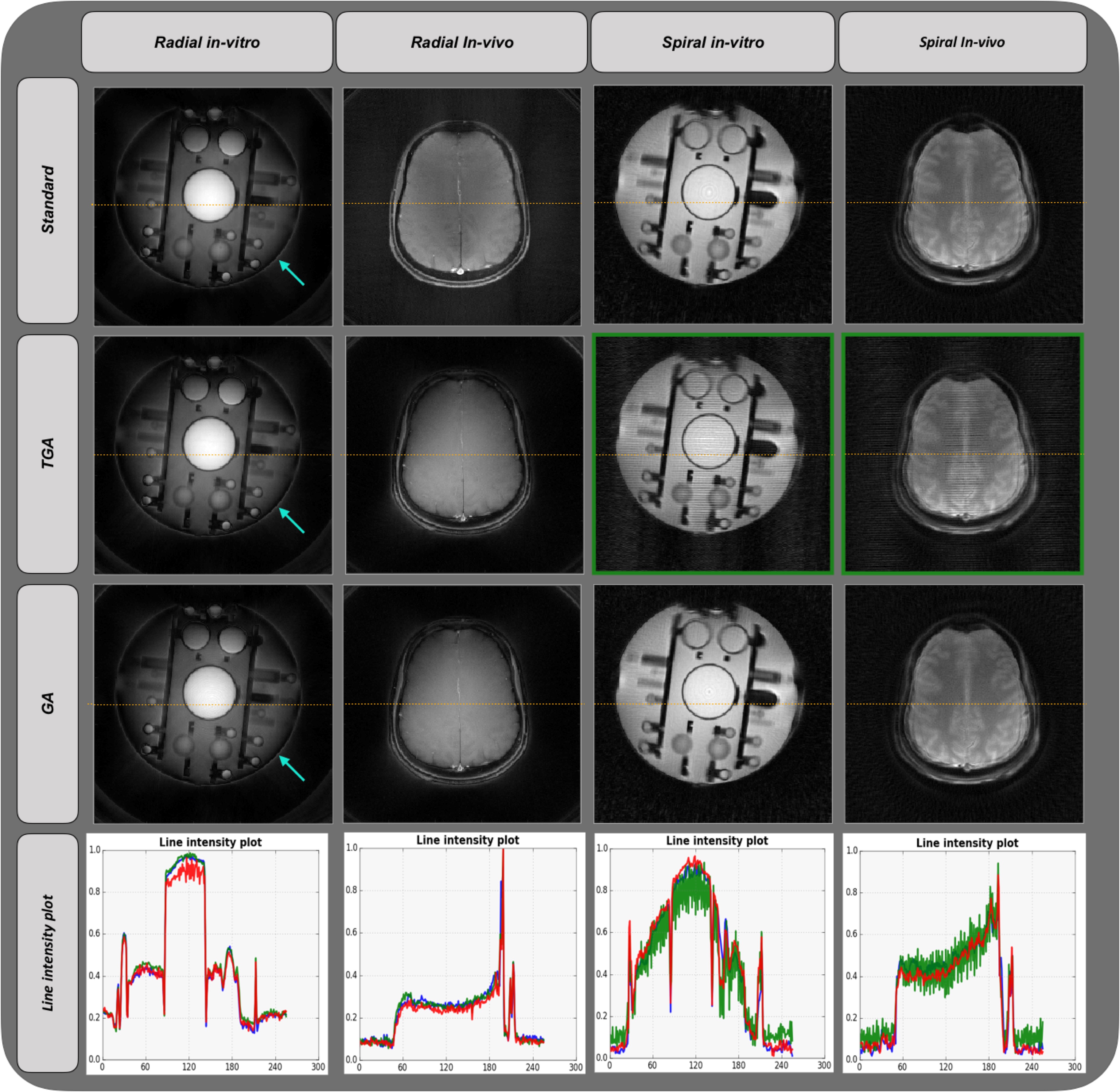
Figure 2 depicts the three variants of radial trajectories (first row) - standard, GA and TGA, gradient waveforms (second row) and representative GRE pulse sequence diagram for 1 TR (third row). Figure 3 shows the three variants of spiral trajectories, representative gradient waveforms and GRE sequence for 1 TR. Figure 4 depicts the reconstructed images in GPI for radial and spiral along with line intensity plot. It can be witnessed from the radial in-vitro images (first column) that there is a bright halo around edges of the phantom (blue arrows). This was due to the delay caused by gradients. The horizontal streaking artefacts can be observed for the images highlighted with green border. The deviation in the line intensity plot (shown with blue arrows) can be observed for spiral in-vitro and in-vivo (TGA) due to the streaking artefact. The SNRs of the reconstructed images are: in-vitro radial with standard, GA and TGA are 32.11dB, 31.17dB and 30.46dB respectively. In-vivo radial with standard, GA and TGA are 30.08dB, 30.64dB and 28.65dB respectively. In-vitro spiral with standard, GA and TGA are 43.90dB, 43.42dB and 30.86dB respectively. In-vivo spiral with standard, GA and TGA are 29.52dB, 28.16dB and 19.29dB respectively.Discussion and Conclusion
ROCKET is a framework that facilitates the researchers for rapid prototyping of MR method development for non-Cartesian based acquisition and reconstruction. This includes trajectory design, pulse sequence design, perform scan upon deploying onto the scanner, image reconstruction and image analysis. ROCKET can be utilized for prototyping and testing other 2D pulse sequences by directly downloading the source-code from GitHub7. Future works includes safety by incorporating peripheral nerve stimulation and specific absorption ratio. It also involves integrating ROCKET to the Pulseq-GPI8 framework as it currently supports Cartesian based acquisition.Acknowledgements
No acknowledgement found.References
1. Layton KJ, Kroboth S, Jia F, Littin S, Yu H, Leupold J, Nielsen JF, Stöcker T, Zaitsev M. Pulseq: A rapid and hardware‐independent pulse sequence prototyping framework. Magnetic resonance in medicine. 2017 Apr;77(4):1544-52. 2. Zwart NR, Pipe JG. Graphical programming interface: a development environment for MRI methods. Magnetic resonance in medicine. 2015 Nov;74(5):1449-60. 3. Delattre BM, Heidemann RM, Crowe LA, Vallée JP, Hyacinthe JN. Spiral demystified. Magnetic resonance imaging. 2010 Jul 1;28(6):862-81. 4. Matthieu Guerquin-Kern, Matlab Code for MRI Simulation and Reconstruction, 2012 5. Wundrak S, Paul J, Ulrici J, Hell E, Rasche V. A small surrogate for the golden angle in time-resolved radial MRI based on generalized fibonacci sequences. IEEE transactions on medical imaging. 2015 Jun;34(6):1262-9. 6. Wundrak S, Paul J, Ulrici J, Hell E, Geibel MA, Bernhardt P, Rottbauer W, Rasche V. Golden ratio sparse MRI using tiny golden angles. Magnetic resonance in medicine. 2016 Jun;75(6):2372-8. 7.https://github.com/imr-framework/imr-framework/tree/MATLAB/MATLAB/ROCKET/Code 8. Ravi KS, Potdar S, Poojar P, Reddy AK, Kroboth S, Nielsen JF, Zaitsev M, Venkatesan R, Geethanath S. Pulseq-Graphical Programming Interface: Open source visual environment for prototyping pulse sequences and integrated magnetic resonance imaging algorithm development. Magnetic resonance imaging. 2018 Oct 1;52:9-15.Figures