2416
Acoustic Noise Reduction Using Digital Filters1Department of Human Biology, University of Cape Town, Cape Town, South Africa, 2Athinoula A. Martinos Centre for Biomedical Imaging, Massachusetts General Hospital, Massachusetts, MA, United States, 3Cape Universities Body Imaging Centre (CUBIC-UCT), University of Cape Town, Cape Town, South Africa, 4MRI Research Unit, University of Tripoli, Tripoli, Libyan
Synopsis
We explored the use of digital low-pass filters to reduce the acoustic noise produced during DTI acquisitions, focusing mainly on the EPI readout. The filters attenuate the high-frequency harmonics of the gradient waveforms which results in
Introduction
Acoustic noise produced during echoplanar imaging (EPI) have been measured to reach 132 dBA.1 High levels of acoustic noise influence functional MRI results2,3, and cause patient discomfort and anxiety. Acoustic noise during MRI acquisitions, which mainly originate from mechanical vibrations in the gradient coil assemblies due to interactions between the rapidly changing currents applied to the coils and the main static field, can be reduced by reducing the spectral content of the gradient waveforms. Modified sinusoidal EPI readouts have previously been proposed.4 In this work, we implement digital filters, focusing on the EPI readout portion of a diffusion weighted imaging (DTI) sequence.Methods
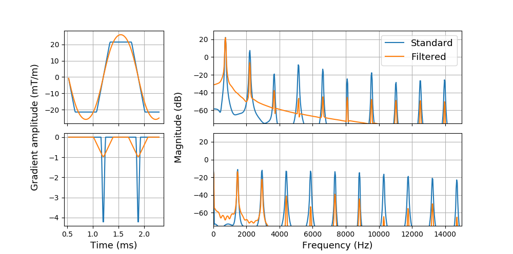
We implemented a digitally-filtered sequence by using a second order Butterworth low-pass filter (LPF) to filter the gradient pulse waveforms, attenuating rather than eliminating4 the harmonics of traditional trapezoidal waveforms. The EPI frequency readout pulse train was filtered with a LPF cut-off frequency (Fc) of 1.5 kHz, attenuating all harmonics (Figure 1, top). Phase encoding blips were widened by 30 μs, causing partial overlap with the ADC sampled region (Figure 1, bottom). In addition to the EPI readout and its associated pre-winders, the crushers around the refocusing radio-frequency (RF) pulses were also filtered using the same digital filter. To correct for the altered k-space trajectory, regridding was performed in the frequency encoding direction only.
Noise levels of (i) the standard sequence, (ii) a sequence with sinusoidal EPI readout and constant phase blip4, and (iii) our digitally-filtered sequence were measured with an Optimic 1155 optical microphone from Optoacoustics, fixed on top of a head coil with a water phantom inside, facing the bore in the right-left direction.
Image quality was assessed in diffusion weighted (DW) images acquired in a healthy volunteer on a 3T Siemens Skyra (Erlangen, Germany) using each of the sequences. Sequence parameters were: TR/TE = 13000/80 ms, 30 gradient directions with b = 1000 s/mm2, five non-DW b=0 s/mm2 volumes, voxel size 2x2x2 mm3. In the digitally-filtered acquisition, the EPI echo spacing of 0.68 ms was increased to 0.73 ms to move the fundamental frequency to a more favourable position on the scanner frequency response function acquired using the method proposed by Wu et al.5 This increase had no effect on TR.
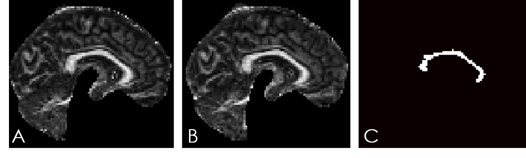
Whole-brain SNR and fractional anisotropy (FA) in the corpus callosum (CC) were compared. Image analysis was performed using open source Python-based software called DIPY (Diffusion Imaging in Python).6 A binary mask of the CC was first generated for each acquisition by applying a threshold of 0.6 to a mid-sagittal slice of the FA map (Figure 4). Masks were multiplied to create a final CC mask (Figure 4 (C)), which was applied to the mid-sagittal slice of each FA map to extract voxelwise FA values across the CC for each acquisition. Voxelwise FA values across the CC were compared using paired t-tests.
Results
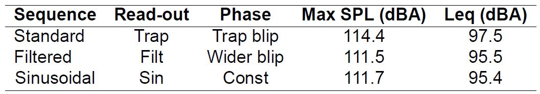
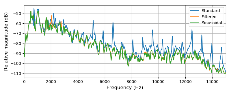
Reductions of 2.9 dBA and 2 dBA for peak sound pressure level (SPL) and equivalent continuous sound level (Leq), respectively, were achieved using the filtered acquisition (Table 1). Results were similar for the sinusoidal version with reductions of 2.7 dBA and 2.1 dBA for peak SPL and Leq, respectively. The acoustic noise spectra of the filtered and sinusoidal DTI sequences demonstrate a significant reduction in EPI harmonics (Figure 2) compared to the standard sequence, but very little difference between each other.
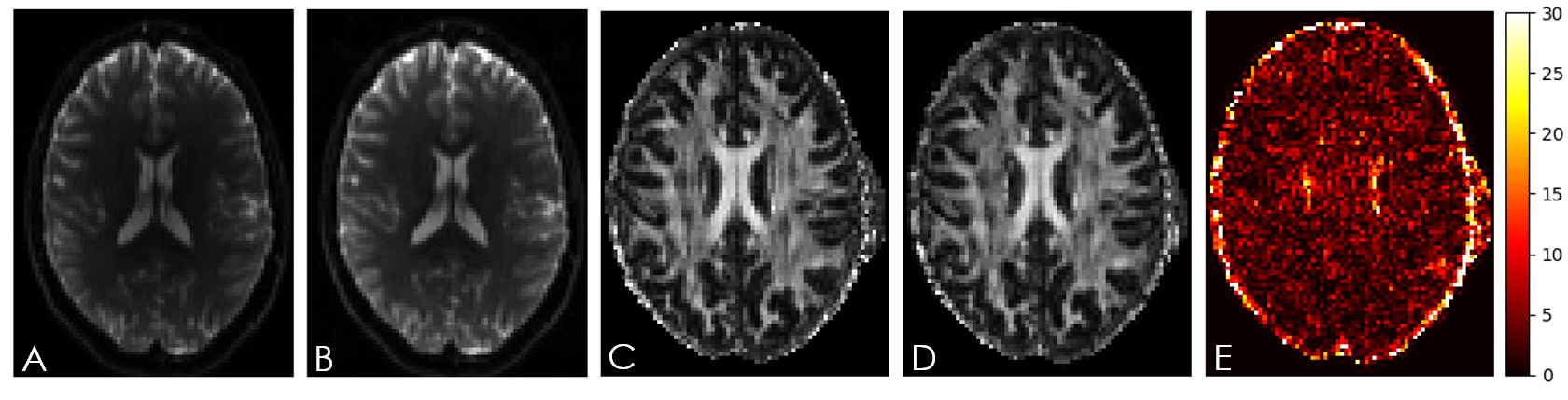
Figure 3 shows b0 images (A and B) and FA maps (C and D) of the same slice, acquired using the standard (A and C) and digitally-filtered (B and D) sequences. The measured whole-brain SNR for the b0 images from the standard (A), digitally-filtered (B), and sinusoidal (not shown) acquisitions were 18.0, 21.4, and 17.17, respectively. Voxelwise FA values in the CC (Figure 4) did not differ between the digitally-filtered and standard acquisitions (t-test, p = 0.77).
Discussion
Filtered EPI readout waveforms showed similar reductions in acoustic noise to the sinusoidal implementation while requiring lower peak amplitudes to produce equivalent moments, with the reduction depending on the filter Fc and EPI echo spacing. The combination of filtered frequency readout waveforms and widened phase encoding blips in contrast to a sinusoidal readout with constant phase blip4 causes less deviation from the standard k-space trajectory leading to increased SNR for the filtered waveforms over the sinusoidal implementation. The proposed method has the potential to be generalized to most gradient waveforms to reduce spectral content and subsequently acoustic noise output.Conclusion
By filtering gradient waveforms, one can effectively reduce the acoustic noise produced during acquisitions with no time penalty or reduction in image quality.Acknowledgements
This work was funded by grants from the National Institutes of Health (R01 HD085813), the South African National Research Chairs Initiative, and the University of Cape Town through the Max & Lillie Sonnenberg Scholarship.References
1. Foster JR, Hall DA, Summerfield AQ, Palmer AR, Bowtell RW. Sound-Level Measurements and Calculations of Safe Noise Dosage During EPI at 3 T. J Magn Reson Imaging. 2000;12(1):157-163.
2. Zhang N, Zhu XH, Chen W. Influence of gradient acoustic noise on fMRI response in the human visual cortex. Magn Reson Med. 2005;54(2):258-263.
3. Tomasi D, Caparelli EC, Chang L, Ernst T. fMRI-acoustic noise alters brain activation during working memory tasks. Neuroimage. 2005;27(2):377-386.
4. Schmitter S, Diesch E, Amann M, Kroll A, Moayer M, Schad LR. Silent echo-planar imaging for auditory FMRI. Magn Reson Mater Physics, Biol Med. 2008;21(5):317-325.
5. Wu Z, Kim YC, Khoo MCK, Nayak KS. Evaluation of an independent linear model for acoustic noise on a conventional MRI scanner and implications for acoustic noise reduction. Magn Reson Med. 2014;71(4):1613-1620.
6. Garyfallidis E, Brett M, Amirbekian B, et al. Dipy, a library for the analysis of diffusion MRI data. Front Neuroinform. 2014;8:8.
Figures