2401
PHASE OFFSET CORRECTION METHODS FOR 7T MRI1Centre for advanced Imaging, University of Queensland, Australia, Brisbane, Australia
Synopsis
At the 7T MRI field, the absence of a volume reference coil results in inter channel phase offsets. It is therefore important to understand the impact of using different phase offset correction methods for producing combined phase images. We quantitatively analysed multi-channel offset corrected 7T GRE-MRI phase images of a phantom obtained using five established methods. Magnetic susceptibility images of a brain were assessed qualitatively in addition. We found that methods which phase offset correct using echo time dependent signal phases contain systematic errors, whereas single echo time methods produce more accurate results.
Introduction
A number of methods have been described in the literature for phase-offset correcting multi-channel MRI phase images. Hammond et al. propose the setting of the phase at the centre voxel of each channel in the imaging volume to zero [1]. Parker et al. create a virtual-reference coil (VRC), generated as a shifted weighted complex sum of the multi-channel signal, and used as a reference for each channel phase [2]. In COMPOSER, the measured phase at a very short echo time is used to correct the phase offset of each channel in the GRE-MRI data [3]. While in MCPC-3D, the offset correction is performed using the phase offsets calculated utilizing multiple echo time GRE-MRI data [4]. We investigate the impact of the choice of the phase offset correction method on combined phase images using a phantom and its impact on QSM images generated from 7T GRE-MRI data in a human brain.Methods
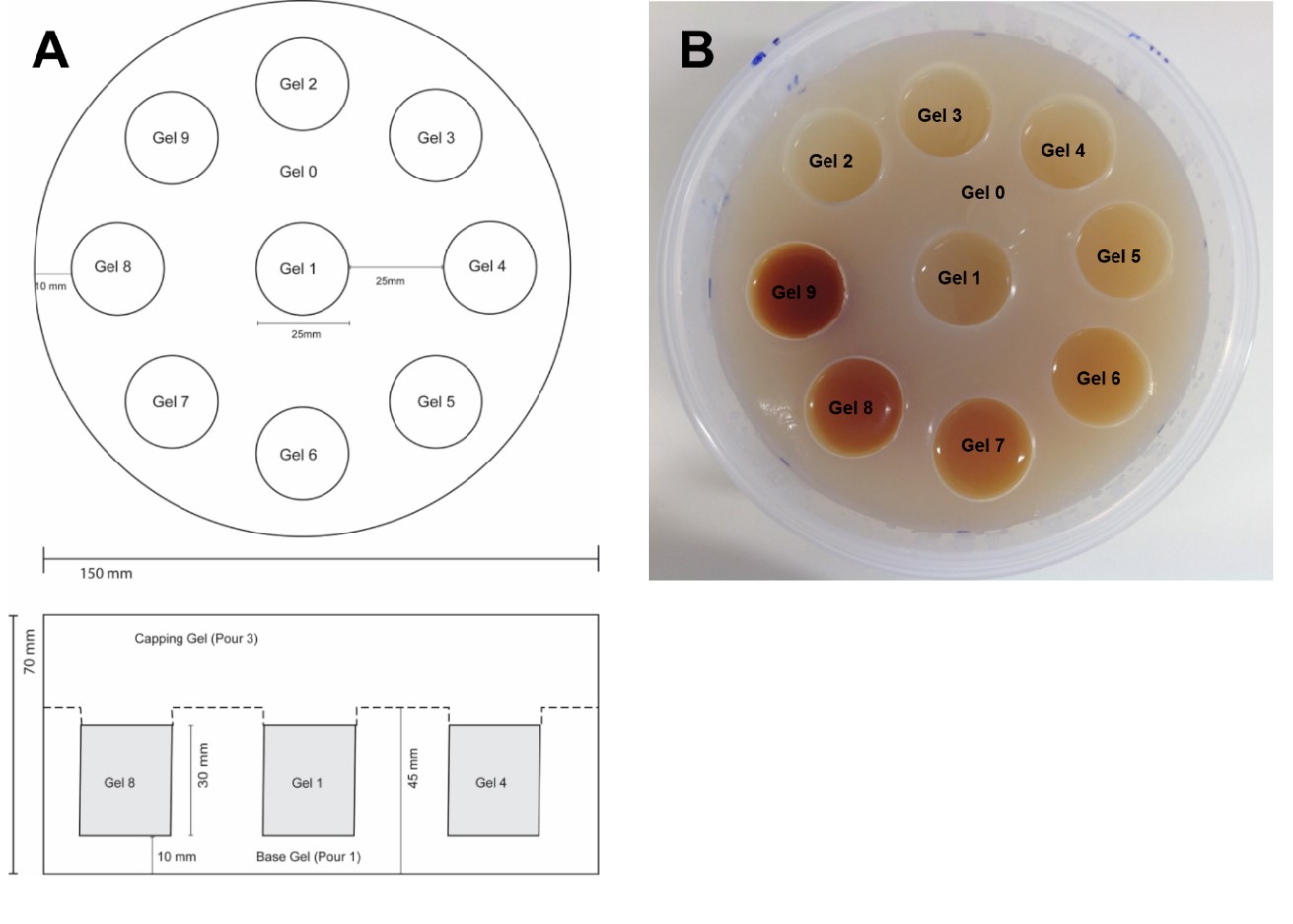
Multi-echo 3D GRE-MRI flow-compensated data were collected for a phantom (Fig. 1) and a male human brain using a whole-body 7T MRI research scanner (Siemens Healthcare, Erlangen, Germany) equipped with a 32-channel head coil (Nova Medical, Wilmington, USA) with the following parameters: TE = 4.4, 7.25, 10.2, 13.25, 16.40, 19.65 and 23ms, TR = 25ms, flip angle = 13o, voxel size = 0.75 x 0.75 x 0.75mm3 and matrix size = 280 x 242 x 128 (phantom) and 280 x 242 x 160 (brain).
We also used a prototype PETRA (Pointwise Encoding Time Reduction with Radial Acquisition) sequence to acquire data for the phantom and brain using the following parameters: TE = 0.07ms, TR = 1.99ms, flip angle = 2o, voxel size = 1 x 1 x 1mm3 and matrix size = 288 x 288 x 288. The multi-echo time multi-channel phase data were phase offset corrected using the following methods:
- Uncorrected: No correction.
- COMPOSER: PETRA-based offset correction. o MCPC-3D: Use 4.4ms and 7.25ms echo time data to offset correct.
- Hammond: Assume centre voxel as reference.
- Parker-8: Use channel 8, the least sensitive channel, as a reference for offset correction (an 11 x 11 region median filter was used on the difference images).
- Parker-12: As in Parker-8, but use the highest sensitivity channel (i.e. 12).
- VRC: Create a virtual reference coil from the channels.
In each case, combined complex images were generated using the sum-of-squares approach. The combined data were used to generate quantitative susceptibility maps (QSM) from the brain data. QSM images were obtained using MRPhaseUnwrap, V-SHARP and iLSQR functions available in STI Suite v2.2 2015 [5, 6] and implemented in MATLAB® 2017b (MathWorks Inc., MA, USA).
Results
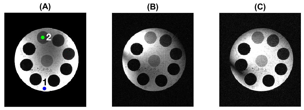
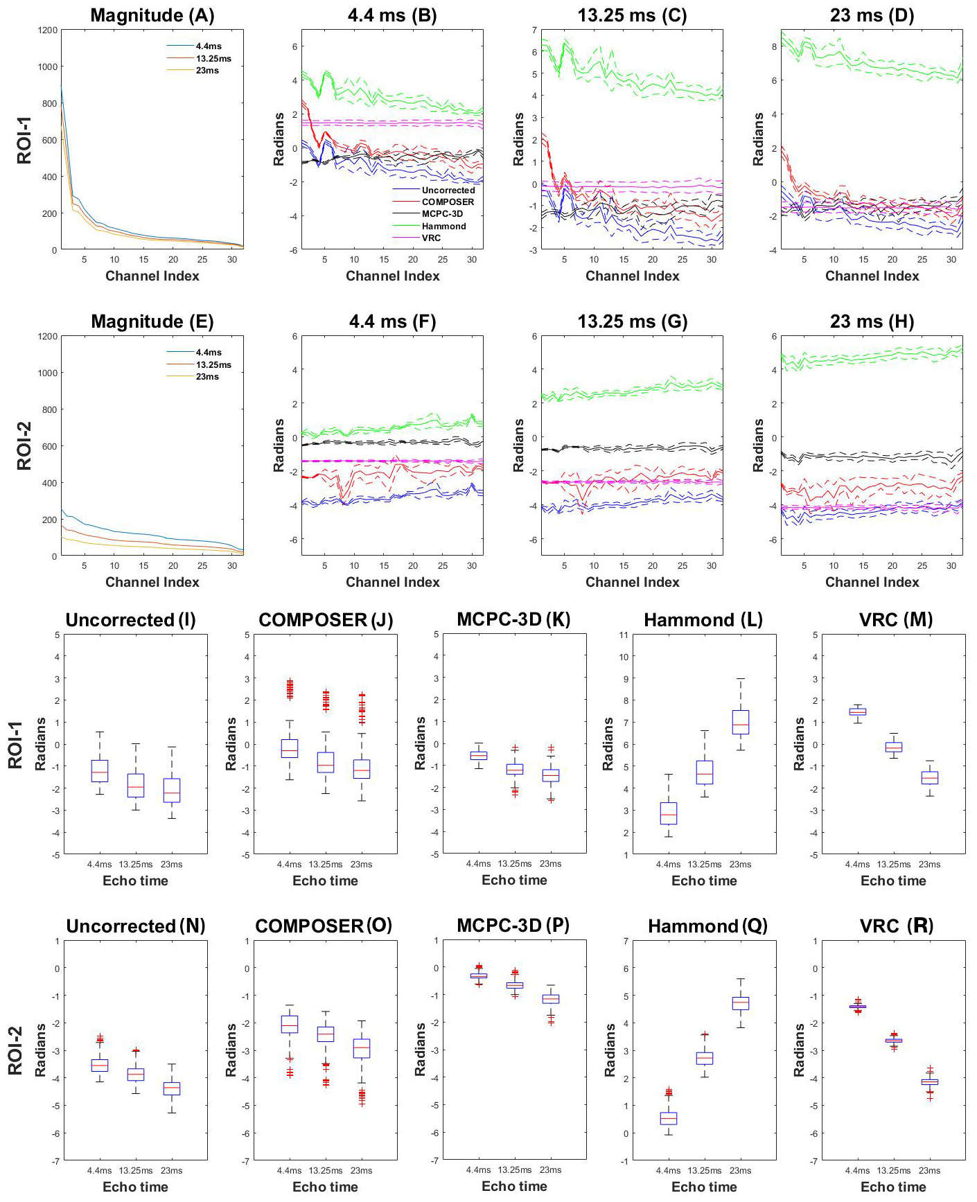
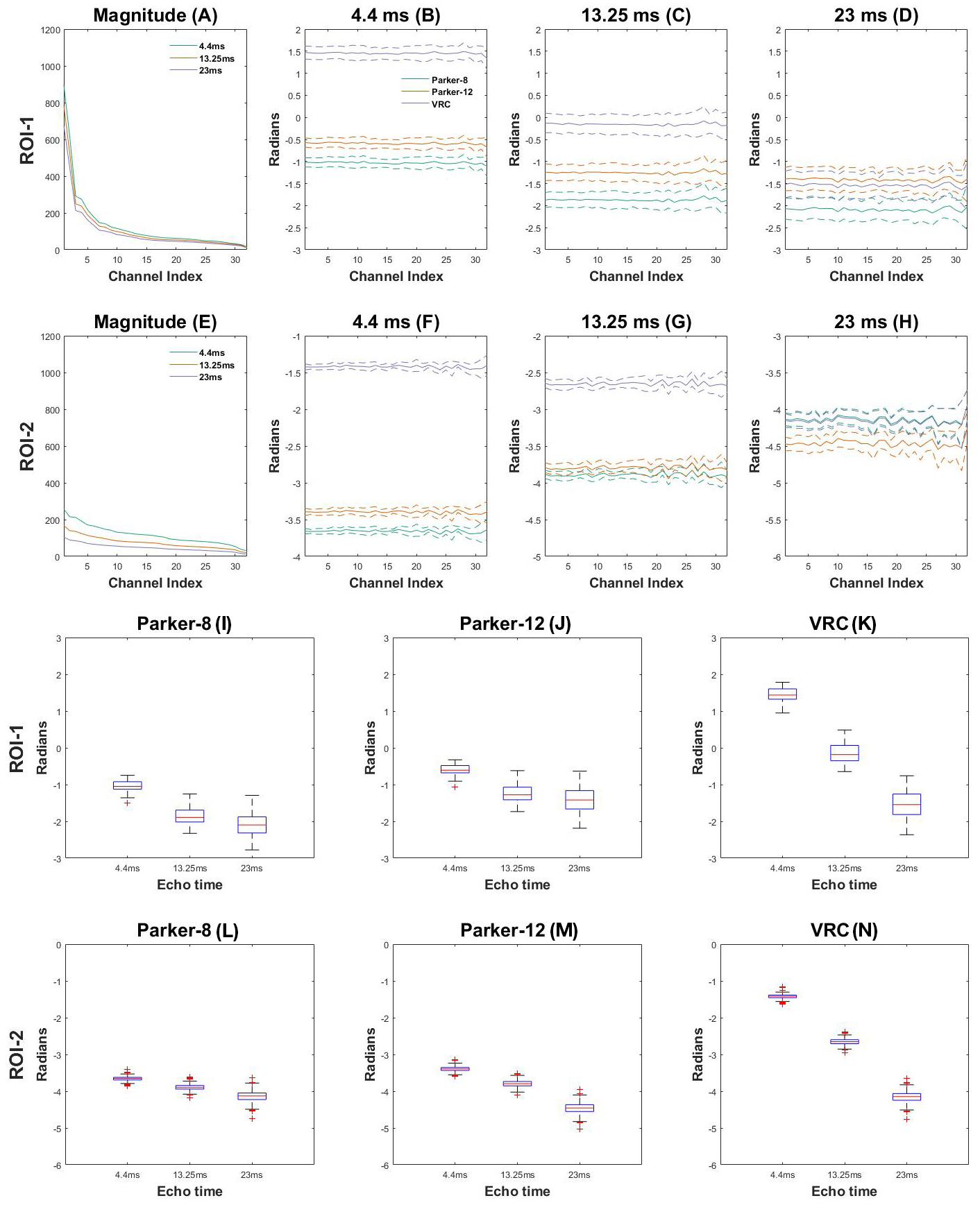
Fig. 3 and 4 provide the results of phase value changes, averaged over a 9 x 9 region, as a function of coil sensitivity measured using the amplitude of signal magnitude for ROI-1 (a region of relatively high signal amplitude variability) and ROI-2 (the low variability region) shown in Fig. 2(A). The VRC method produced the least amount of variability as a function of channel.
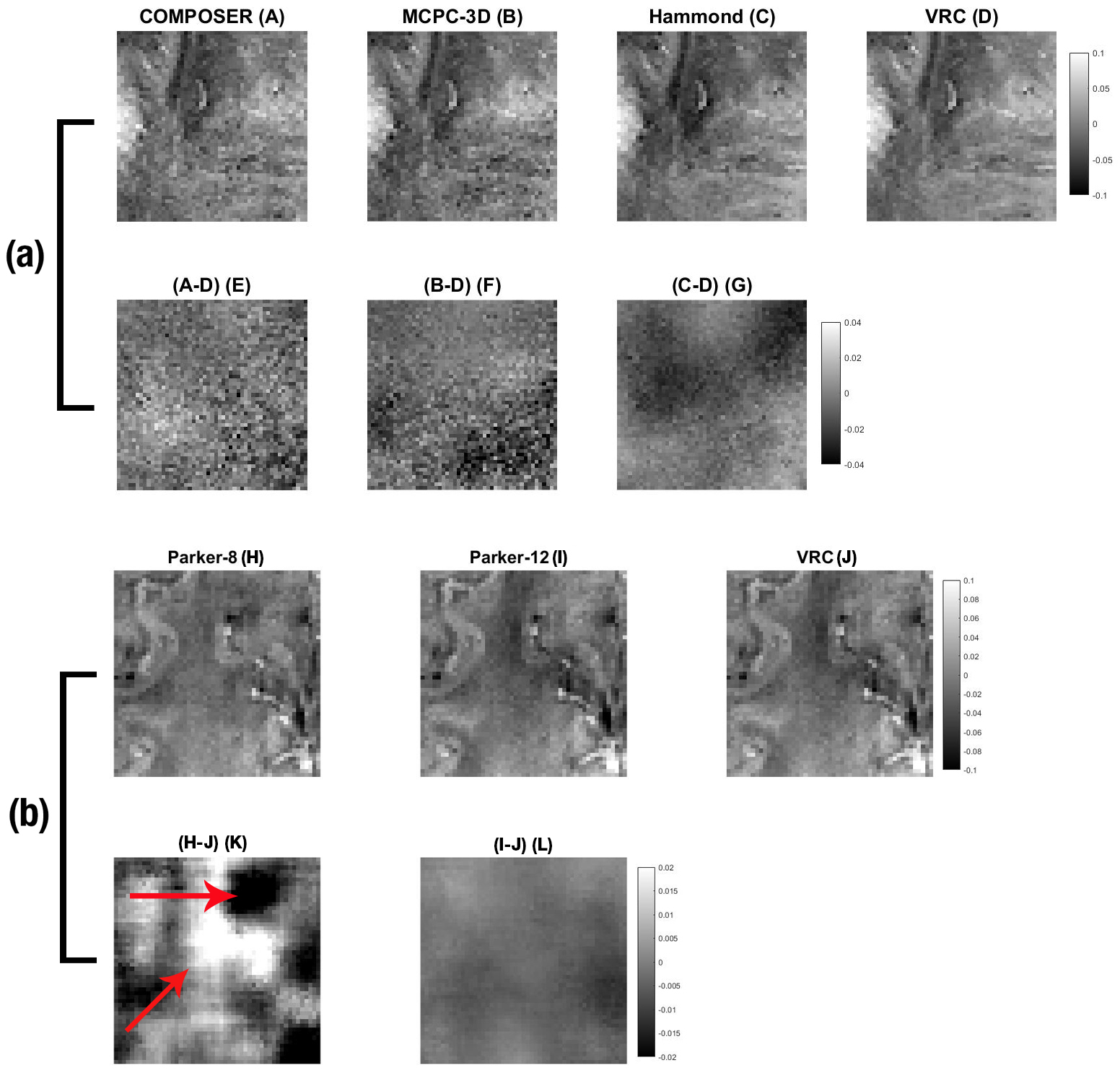
Fig. 5 provides zoomed-in results for two selected regions within the brain. COMPOSER and MCPC-3D methods were found to perform similarly, with the Hammond method producing generally less noisy results. From Fig. 4 we conclude that the impact of the choice of the reference may not necessarily deteriorate the quality of phase offset correction, but from Fig. 5 we can infer that the effect is non-trivial on the quality of QSM results. Overall, the quality of the VRC produced QSM images appears to be better than others.
Discussion
COMPOSER and MCPC-3D assume phase values evolve linearly with echo time, which may not hold in grey and white matter [7-10]. Whilst the method of Hammond et al. is computational efficient, the VRC approach was able to produce higher quality images [1, 2].
We have analysed how the choice of a certain coil for reference change the result with respect to the VRC method and we conclude that in cases involving receiver coils with dissimilar coil sensitivity profiles (Parker-8 for low, and Parker-12 for high), single-channel referencing could be used as a viable method for producing VRC quality images without the computational cost associated with deriving the virtual reference coil.
Conclusion
Our study suggests that phase offset correction can systematically influence combined phase images. We found the VRC method to lead to the most robust combined phase images and QSM results. Ultra-high field MRI studies relying on GRE-MRI signal phase should consider the impact of the choice of the phase offset correction method employed.Acknowledgements
The authors would like to acknowledge the use of the USPIO doped gel phantom developed by Greg Brown for his study reported in [11] and the facilities of the National Imaging Facility at the Centre for Advanced Imaging, The University of Queensland. The authors would like to thank the National Health and Medical Research Council (NHMRC APP1104933, Australia) for partially funding the project.References
[1] K. E. Hammond, J. M. Lupo, D. Xu, M. Metcalf, D. A. Kelley, D. Pelletier, et al., "Development of a robust method for generating 7.0 T multichannel phase images of the brain with application to normal volunteers and patients with neurological diseases," Neuroimage, vol. 39, pp. 1682-1692, 2008.
[2] D. L. Parker, A. Payne, N. Todd, and J. R. Hadley, "Phase reconstruction from multiple coil data using a virtual reference coil," Magnetic Resonance in Medicine, vol. 72, pp. 563-569, 2014.
[3] S. D. Robinson, B. Dymerska, W. Bogner, M. Barth, O. Zaric, S. Goluch, et al., "Combining phase images from array coils using a short echo time reference scan (COMPOSER)," Magnetic resonance in medicine, 2015.
[4] S. Robinson, G. Grabner, S. Witoszynskyj, and S. Trattnig, "Combining phase images from multi‐channel RF coils using 3D phase offset maps derived from a dual‐echo scan," Magnetic resonance in medicine, vol. 65, pp. 1638-1648, 2011.
[5] S. M. Smith, M. Jenkinson, M. W. Woolrich, C. F. Beckmann, T. E. Behrens, H. Johansen-Berg, et al., "Advances in functional and structural MR image analysis and implementation as FSL," Neuroimage, vol. 23, pp. S208-S219, 2004.
[6] W. Li, A. V. Avram, B. Wu, X. Xiao, and C. Liu, "Integrated Laplacian‐based phase unwrapping and background phase removal for quantitative susceptibility mapping," NMR in Biomedicine, vol. 27, pp. 219-227, 2014.
[7] S. Wharton and R. Bowtell, "Fiber orientation-dependent white matter contrast in gradient echo MRI," Proceedings of the National Academy of Sciences, vol. 109, pp. 18559-18564, 2012.
[8] P. Sati, P. van Gelderen, A. C. Silva, D. S. Reich, H. Merkle, J. A. De Zwart, et al., "Micro-compartment specific T 2⁎ relaxation in the brain," Neuroimage, vol. 77, pp. 268-278, 2013.
[9] M. J. Cronin, N. Wang, K. S. Decker, H. Wei, W.-Z. Zhu, and C. Liu, "Exploring the origins of echo-time-dependent quantitative susceptibility mapping (QSM) measurements in healthy tissue and cerebral microbleeds," NeuroImage, vol. 149, pp. 98-113, 2017.
[10] S. Sood, J. Urriola, D. Reutens, K. O’Brien, S. Bollmann, M. Barth, et al., "Echo time‐dependent quantitative susceptibility mapping contains information on tissue properties," Magnetic resonance in medicine, 2016.
[11] G. C. Brown, G. J. Cowin, and G. J. Galloway, "A USPIO doped gel phantom for R2* relaxometry," Magnetic Resonance Materials in Physics, Biology and Medicine, vol. 30, pp. 15-27, 2017.
Figures