2349
An analysis of post-processing steps for residue function dependent DSC-MRI biomarkers through their clinical impact on glioma diagnosis for both 1.5 and 3T1Barrow Neurological Institute, Phoenix, AZ, United States
Synopsis
Several recent initiatives have focused on optimizing and standardizing DSC-MRI imaging protocols and post-processing steps. With the availability of public imaging databases that include clinical outcomes, various post-processing steps can be carefully assessed for their impact on the clinical outcomes. Here we evaluated post-processing steps for advanced perfusion biomarkers that relay on determining the residue function by examining the clinical impact of each step. In summary we determined that updating the current deconvolution steps is beneficial, and that normalization allows for tumor grading across clinical field strengths.
Introduction:
Dynamic susceptibility contrast (DSC) MRI based cerebral blood volume (CBV) has been shown to improve clinical care for brain tumor patients. Advanced biomarkers such as cerebral blood flow (CBF), mean transit time (MTT), and capillary transit heterogeneity (CTH) may be better indicators of microvascular flow abnormalities, but are less commonly used because they involve more complex post-processing in order to estimate the residue function. The goal of this study is to compare the influence of deconvolution methods on residue function and CTH fidelity and their clinical impact on glioma grading at both 1.5 and 3T.Methods:
Clinical dataset: This retrospective study utilizes a publicly available dataset1 on The Cancer Imaging Archive. This “Glioma DSC-MRI Perfusion Data” dataset contains 49 co-registered T1-weighted SPGR and DSC-MRI images of low (n = 13) and high grade (n = 36) glial brain lesions. These MRI images were acquired on both 1.5T (n = 26) and 3T (n = 23) field strengths. A preload of 0.05 mmol/kg of gadobenate dimeglumine was used. This dataset also provided regions-of-interest (tumor, arterial input function (AIF), and normal-appearing-white-matter (NAWM) as segmented by a radiologist).
Residue Function Determination: We evaluated two deconvolution methods, including one that employs circular2 discretization of the AIF followed by a truncated3 singular value decomposition (SVD) while the other relies on Volterra4 discretization of the AIF followed by standard-form Tikhonov regularization with L-curve criterion5. The first method (Method 1) is the most commonly used approach in the field and aims to minimize oscillations in the residue function brought on by the discretization method. The later approach (Method 2) has been recommended by a highly-cited paper6 in the DSC community, but has been slow to be integrated. We also investigated the impact of applying the Boxerman-Schmainda-Weiskoff7 (BSW) method and biomarker normalization.
Biomarker Calculations: Once the residue function was determined by the methods outlined above, CBF was determined to be the maximum value of the residue 3. A gamma-variate function was then fit to the residue function, and parameters8 were computed using MTT = αβ and CTH = β√α.
Statistics: The ability for each biomarker to distinguish and classify between tumor grade was evaluated using two statistical tests. Since data were acquired over different field strengths and vendors, we first performed a multiway ANOVA for field strength, vendor, and tumor grade differences. Biomarkers that did not statistically depend on field strength or vendor were then evaluated for their ability to classify tumor grade using Receiver Operating Characteristics (ROC) analysis. The AUROC (area under the ROC) is reported, along with the 95% upper and lower confidence intervals (CI) and the optimal threshold that maximizes sensitivity and specificity. A p-value < 0.05 was considered significant for all statistical tests.
Results and Discussion:
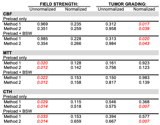
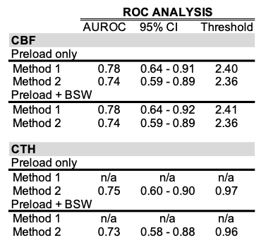
Table 1 summaries the p-values from the multi-way ANOVA tests. In general, the application of BSW did not change any of the statistical results. Unnormalized MTT was statistically different across field strengths for both methods, and even once normalized no statistical difference was seen between tumor grade. Unnormalized and normalized CBF was not statistically different across field strength, but only showed a statistical difference between tumor grade when normalized to NAWM for both methods (p-value = 0.017 and 0.039, respectively). Unnormalized CTH was statistically different across field strength for both methods, but once normalized to NAWM was not. However, only method 2 was able produce a statistical difference for tumor grade (p-value = 0.007 for both preload only and preload w/BSW). For the combination of processing steps that did not result in a field strength dependency and was able to distinguish low from high tumor grade, ROC analysis was conducted (Table 3). Here we see similar ROC results for both the preload only and preload w/BSW cases. Additionally, the AUROC of the CTH calculated by Method 2 is similar to previously AUROC reported9 when CTH is calculated with Bayesian estimation.Conclusion:
Bayesian estimation is the most common technique for CTH computation, but is computational demanding. However, in this study, updating the traditional approaches to solving the SVD deconvolution showed promise. Of the more advanced biomarkers, both CBF and CTH benefited from being calculated with Method 2, indicating that Volterra discretization and L-curve regularization is a robust approach for advanced DSC-MRI brain tumor analysis. Future work encompasses examining the effects of pre-processing steps such as thresholding and filtering, and NAWM segmentation approaches.Acknowledgements
Research supported by R01 CA158079-01.References
[1] Schmainda KM, Prah MA, Connelly JM, Rand SD. (2016). Glioma DSC-MRI Perfusion Data with Standard Imaging and ROIs. The Cancer Imaging Archive.[2] Wu O, Østergaard L, Weisskoff RM, Benner T, Rosen BR, Sorensen AG. Tracer arrival timing-insensitive technique for estimating flow in MR perfusion-weighted imaging using singular value decomposition with a block-circulant deconvolution matrix. Magn. Reson. Med. 2003;50:164–74.[3] Østergaard L, Weisskoff RM, Chesler DA, Gyldensted C, Rosen BR. High resolution measurement of cerebral blood flow using intravascular tracer bolus passages. Part I: Mathematical approach and statistical analysis. Magn. Reson. Med. 1996;36:715–725.[4] Sourbron S, Luypaert R, Morhard D, Seelos K, Reiser M, Peller M. Deconvolution of bolus-tracking data: a comparison of discretization methods. Phys. Med. Biol. 2007;52:6761–78.[5] Sourbron S, Dujardin M, Makkat S, Luypaert R. Pixel-by-pixel deconvolution of bolus-tracking data: optimization and implementation. Phys. Med. Biol. 2007;52:429–47.[6] Willats L, Calamante F. The 39 steps: evading error and deciphering the secrets for accurate dynamic susceptibility contrast MRI. NMR Biomed. 2013;26:913–93.1[7] Boxerman JL, Schmainda KM, Weisskoff RM. Relative cerebral blood volume maps corrected for contrast agent extravasation significantly correlate with glioma tumor grade, whereas uncorrected maps do not. AJNR. Am. J. Neuroradiol. 2006;27:859–67.[8] Mouridsen K, Hansen MB, Østergaard L, Jespersen SN. Reliable estimation of capillary transit time distributions using DSC-MRI. J Cereb Blood Flow Metab. 2014;34(9):1511-21.[9] Tietze A, Mouridsen K, Lassen-Ramshad Y, Østergaard L. Perfusion MRI Derived Indices of Microvascular Shunting and Flow Control Correlate with Tumor Grade and Outcome in Patients with Cerebral Glioma Najbauer J, editor. PLoS One 2015;10:e0123044.Figures