Synopsis

A new user interactive platform for MRS data processing is proposed. This toolbox is based on the Semi-Classical Signal Analysis (SCSA) for Residual Water Suppression and MRS signal denoising. It allows MRS users to achieve water suppression and data denoising, with data fitting as an additional feature. The toolbox is easy to install and to use: 1) visualization of spectroscopy data, 2) water suppression and denoising, 3) iterative data fitting using nonlinear least squares. This abstract demonstrates how each of these features has been incorporated and provides technical details about the implementation as a graphical user interface in MATLAB.

Introduction

Signal analysis methods like Hankel Lanczos Singular Value Decomposition (HLSVD)¹ and the HLSVD with Partial Re-Orthogonalization (HLSVD-PRO) ² have been proposed as post-processing techniques for residual water suppression. We have introduced the SCSA-based Matlab toolbox considering its effectiveness to suppress residual water and increase the Signal-to-Noise Ratio (SNR) in the $$$^1$$$H-MRS data. The toolbox offers the following operations on an unsuppressed water MRS data: 1. visualization of a single voxel and multi-voxels MRS data in time and frequency domain 2. pre-processing of MRS data with phase correction, apodization along with water suppression and denoising using SCSA 3. robust time-domain fitting routine (the advanced method for accurate, robust and efficient spectral fitting (AMARES) algorithm³.

Methods

The toolbox, developed in MATLAB, for $$$^1$$$H-MRS data analysis, is straight forward and for immediate use. It can be run immediately after installation, with no requirements.

1. Importing data

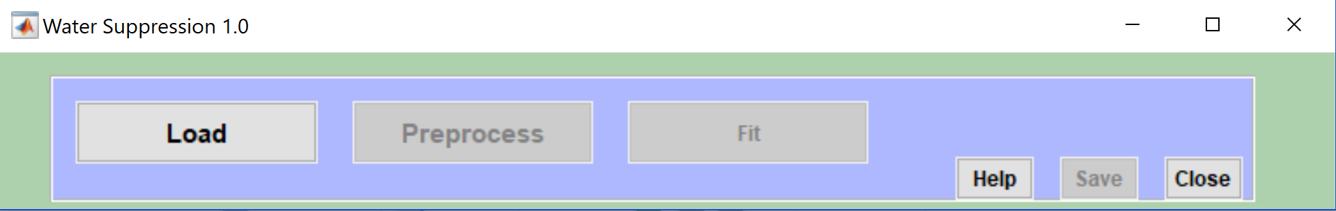
This software can load only raw data (.mat file) according to the following structure with the variables, complex_fid_unsuppressed being complex time domain single or multi voxel water unsuppressed signal, and $$$Fs$$$ being the sampling frequency. The main window of the toolbox is shown in Figure 1

1. Pre-processing module

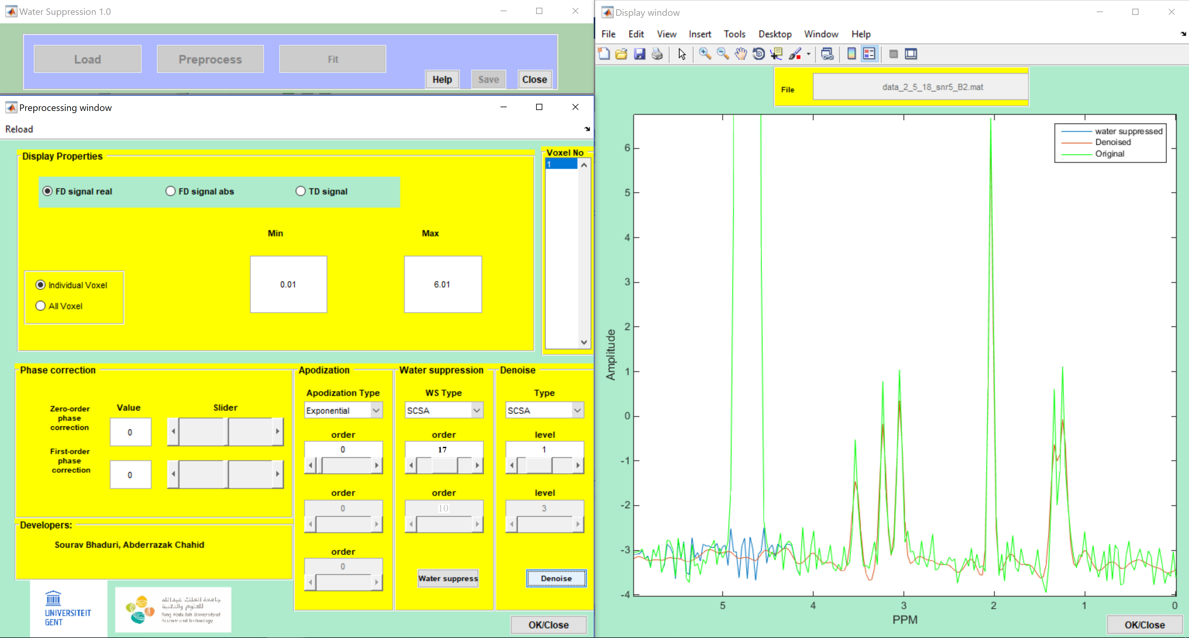
Once loading the data, the Preprocess button in the main window can be used to perform a voxel by voxel phase correction, apodization, water suppression and data denoising. A Display window will open in parallel to the Preprocessing window (Figure 3). The display segment can be changed by changing the display ppm range in the Display Properties panel at the top of the Preprocessing window. Zero-order phase correction can be used to perform zero-order and first-order phase correction by moving the slider inside the Phase correction panel. The Apodization panel can perform apodization on the data with Exponential, Gaussian, Gaussian-Exponential, and Sigmoid functions. Water suppress panel will suppress water peak, voxel wise, using the SCSA method by selecting the desired number of eigenfunctions (default value: $$$\mathbf{17}$$$) which can be entered directly or using the slider. The denoising level set by the SCSA parameter $$$h$$$ (default value: $$$\mathbf{1}$$$) can be entered directly or using the slider.

2. SCSA-based Pre-processing

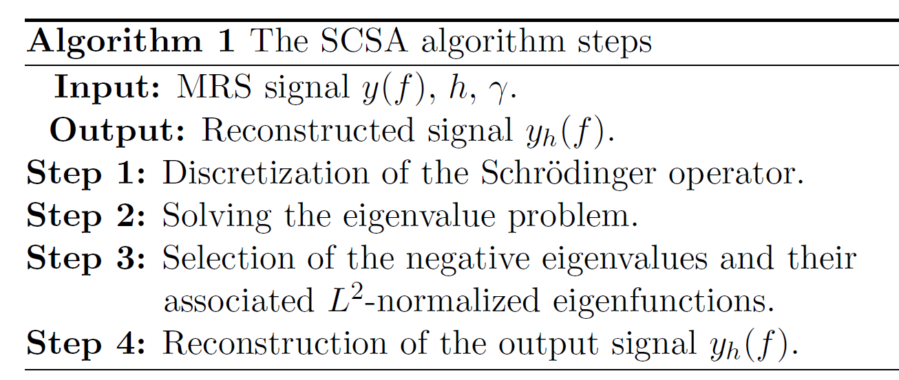
The proposed SCSA method is embedded in this toolbox. For a given $$$h$$$, the approximated signal $$$y_{h}(f)$$$ of the original MRS signal $$$y(f)$$$ is given by: \begin{equation} y_{h}(f) = 4h \displaystyle \sum_{k=1}^{N_{h}} \sqrt{\left(-\mu_{kh} \right)}~ {\psi}^{2}_{\,kh}(f) \end{equation} where $$$h$$$ is a positive constant, $$${\mu}_{kh}$$$ and $$${\psi_{kh}(f)}$$$, for $$$k= 1,\cdots, N_h $$$, refer to the negative eigenvalues and associated eigenfunctions of $$$ H(y) $$$ defined by: \begin{equation}\label{Sch_prob1} H(y) { \psi(f)}= -h^2~ \frac{d^{2} \psi(f)}{d^{2}f} - y(f)~\psi(f) = \mu \, {. \psi(f)}. \end{equation} The SCSA method described by the algorithm given in Figure 2 is used for two different purposes:

• Residual water suppression: Reconstruct the water peak using a minimum number of eigenfunctions with an optimal choice of $$$h$$$. Removes the remaining eigenfunctions representing the rest of the spectrum (e.g: metabolites, noise...) to recover only the water peak⁴.
• MRS denoising: Separate the useful information from the noise by an optimal choice of $$$h$$$ based on SNR maximization and preservation of the peak areas of the metabolites⁵.

3. Fitting and output module

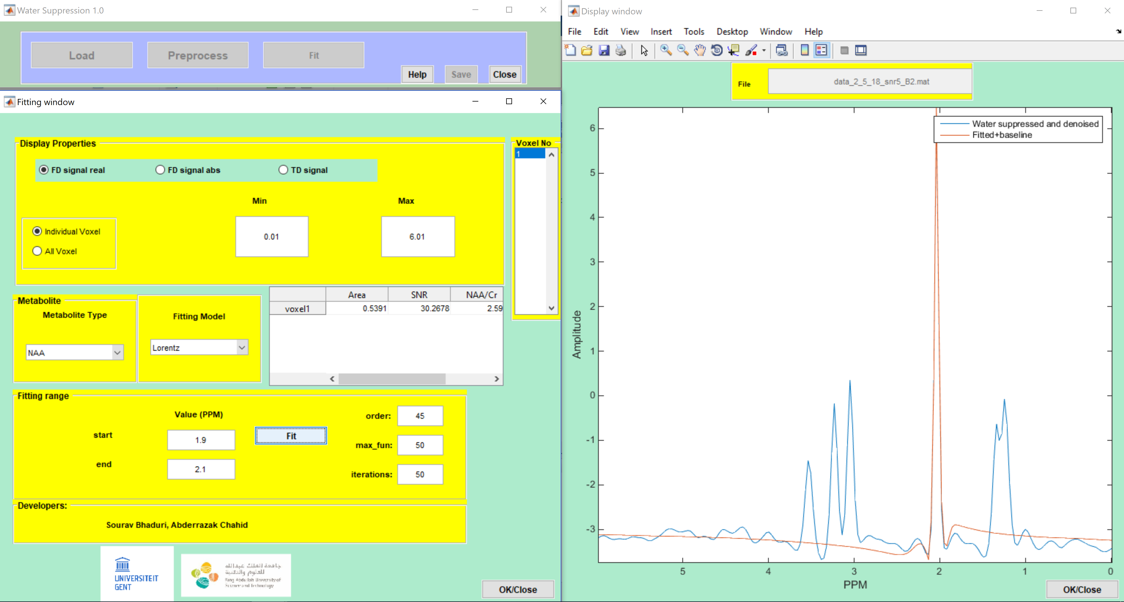
The fitting algorithm is based on AMARES method, with Lorentz, Gauss, and Voigt model functions. The Fitting window, shown in Figure 4, allows for AMARES parameter setting. Fitting is performed once the peaks are selected from the Metabolite panel. The output variables: fitted peak area, SNR, NAA/Cr, and Cho/Cr, error in fitting (Cramer-Rao bound in $$$\%$$$ of quantified peak amplitude) are displayed in the first five columns of a table right to the Metabolite panel. These results could be saved with the save button. An output excel file is generated as the ‘main file name_output.csv’ containing all the output variables of interest.

Discussion and Conclusion

Acknowledgements

References

1. Pijnappel W, Van den Boogaart A, De Beer R, Van Ormondt D. SVD-basedquantification of magnetic resonance signals. Journal of Magnetic Resonance(1969). 1992;97(1):122–134.

2. Laudadio T, Mastronardi N, Vanhamme L, Van Hecke P, Van Huffel S. ImprovedLanczos algorithms for blackbox MRS data quantitation. Journal of magneticresonance (San Diego, Calif : 1997). 2002;157:292–7.

3. Vanhamme L, van den Boogaart A, Van Huffel S. Improved method for accurateand efficient quantification of MRS data with use of prior knowledge. Journal ofMagnetic Resonance. 1997;129(1):35–43

4. Chahid A, Serrai H, Achten E, Laleg‐Kirati TM. Magnetic Resonance Spectroscopy data water suppression using squared siegnfunctions of the Schrodinger operator. ESMRMB held in Barcelona/ES from October 19 - October 21, 2017.

5. Laleg‐Kirati TM, Zhang J, Achten E, Serrai H. Spectral data de‐noising using semi‐classical signal analysis: application to localized MRS. NMR in Biomedicine. 2016 Oct;29(10):1477-85.