2231
Optimal Analysis Strategies for GABA Quantification with 1H J-Edited MRS1Neurology, University of California, Los Angeles, Los Angeles, CA, United States, 2Advanced Imaging Research Center, University of Texas Southwestern Medical Center, Dallas, TX, United States, 3NeuroSpectroScopics LLC, Sherman Oaks, CA, United States, 4Psychiatry and Biobehavioral Sciences, University of California, Los Angeles, Los Angeles, CA, United States
Synopsis
This study evaluated
the performance of 9 unique methods of deriving GABA and GABA+ from J-edited-single-voxel-MRS
using a set of high-quality spectra obtained from the anterior middle cingulate
cortex in 34 pediatric human subjects. The results indicate that spectral
integration produces the most consistent between-subject measure of GABA+ and
that non-linear least-squares fitting that includes macromolecule confound
spectral models together with GABA spectral models best produces the expected
positive correlation between voxel gray matter content and GABA.
Introduction
J-Edited-Single-Voxel-MRS is in common use for detecting/quantifying brain γ-amino-butyric-acid (GABA), although there remains uncertainty about how to optimally derive the GABA level from such studies. In particular, brain macromolecules (MMs) produce confounding co-edited signals leading to the custom of reporting GABA+ (= GABA + MM) rather than GABA. This work compared the performance of nine GABA analysis/quantification approaches with emphasis on determining whether non-linear-least-squares spectral fitting using custom metabolite and MM baseline (MMBL) spectral models might be helpful for GABA quantification.Methods
J-edited spectra were acquired as part on an ongoing MRI/MRS study of awake children (aged 90–160 months) who had diagnoses of ADHD+PAE (Attention Deficit Hyperactivity Disorder with Prenatal Alcohol Exposure) or ADHD-PAE (ADHD without PAE) or were normally developing controls. GABA+ J-Edited-MRS without MM suppression (12.0 cm3 voxel size, 32-channel receive-phased-array, TR/TE/av=2000/68/128, unmodified investigational 859G Works-In-Progress package) was performed with a Siemens 3T Prisma MRI unit (Figure 1). MRS voxels were positioned in the anterior Middle Cingulate Cortex (aMCC) (Figure 2). Not-Water-Suppressed (NWS) spectra (av=8) were also obtained. Acquired spectra were visually reviewed for artifacts (subtraction errors, phase errors, large lipid, motion) to identify 34 high-quality acquisitions from unique subjects. 3D-T1w imaging was also performed. The T1w volumes were segmented into GM, WM and CSF subvolumes. MRS voxels were overlaid onto the subvolumes to determine the fraction of GM, WM and CSF within each voxel (Figure 2).
The J-edited-difference-spectrum (DIFF) and the off-resonance-control-spectrum (OFF) were analyzed using analysis approaches M0 – M8. Unless otherwise indicated, all GABA endpoints were NWS-water-referenced (WR) and corrected for CSF content (CSFC).
M0: Integration using custom-written software (PySINT) of the DIFF 3.0±0.5 ppm region and the NWS OFF 4.69±0.5 ppm region to obtain a water-referenced GABA+ ratio measure.
M1: LCModel (LCM) fitting of OFF (0.0 – 4.0 ppm) using standard LCM TE68 spectral models.
M2: LCM fitting of DIFF (1.9 – 4.2 ppm) using custom LCM spectral models.
M3: LCM fitting of DIFF as in M2, except the GABA endpoint was expressed as GABA:CrT (Cr-referenced rather than WR), where CrT (creatine+phosphocreatine) was obtained from M1.
M4: Fitting the DIFF 2.75 - 4.00 ppm region with SVFit2016 (SVF) software using VESPA (Versatile Simulation, Pulses and Analysis (https://pypi.org/project/Vespa-Suite/)) generated GABA and glutamate-glutamine spectral models.
M5: SVF fitting the OFF (0.0 – 4.00 ppm) using VESPA-generated spectral models.
M6: SVF fitting as in M4 with the addition of a flexible 2.75 – 3.25 ppm MMBL model. (The shape of the MMBL signal could be fitted differently for each study.)
M7: SVF fitting as in M6, except using a rigid MMBL model shape that was an amalgamated but rigid version of the M6 best fit MMBL shapes.
M8: SVF fitting as in M6, except using a rigid MMBL model shape that was derived from Mikkelsen et al1
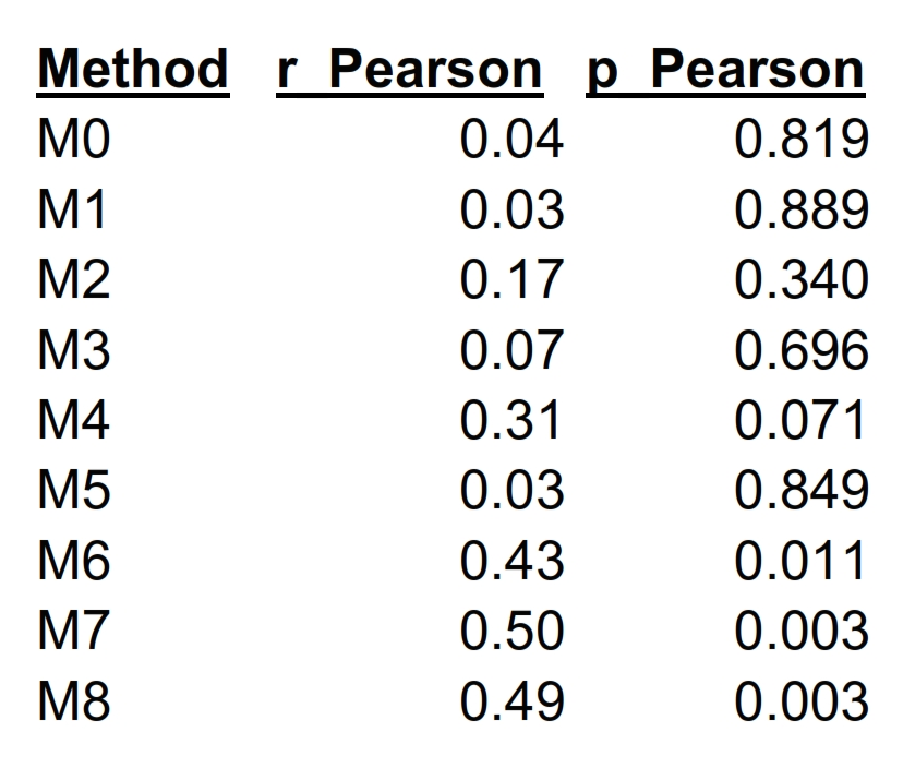
Performance of the 9 methods was assessed by comparing 1) the
between-subject coefficient of variation (COV) for the GABA endpoints and 2) the
GM vs GABA (Pearson) correlations produced by each method. It was assumed that
an optimally performing method would minimize COV and maximize (positive) GM vs
GABA correlation because GABA is more concentrated in GM compared to WM and CSF.2
Results
No differences in performance between the PAE+ADHD, PAE-ADHD and Control groups were apparent and the groups were merged for further analysis. Between-subject COVs for each method are given in Table 1. Signal integration (M0) produces optimal performance in terms of minimizing COV. However M0 has the disadvantage of producing a GABA+ endpoint. All other procedures (M1-M8) used GABA and MMBL spectral models seeking to fit GABA independently of MMBL to produce a better estimate of GABA. DIFF fitting (M2-M4 and M6-M8) showed better COV performance in comparison to OFF fitting (M1 and M5). This was hypothesized because J-editing removes many GABA overlapping signals, however this hypothesis appears to have not yet been tested with 3T data. Cr-referencing (M3), as advocated by Mikkelsen et al1, performed similarly to NWS-water-referencing (M2). Two separate software packages (SVF and LCM) showed similar performance (M2 vs M4). MMBL model inclusion worsens COV performance (M2-M4 vs M6-M8). However Table 2 and Figure 3 show that MMBL model inclusion enhances the probability of detecting a GM vs GABA correlation. M6-M8 produced statistically significant positive GM vs GABA correlations.Summary
This contribution illustrates that multiple analysis methods can be used to derive GABA from J-edited-spectra. Including a MMBL model when fitting a J-edited difference spectrum helps to separately quantify MMBL and GABA (as opposed to GABA+) although COVs on the order of 25-35% should be anticipated.Acknowledgements
Financial support from NIH AA025066References
1. Mikkelsen et al. NeuroImage 2017; 159: 32-45.
2. Mikkelsen et al. NMR Biomed 2016; 29: 1644-1655.
Figures