2191

Improved Quantification for Steady-Pulsed ASL Perfusion Imaging

NAM GYUN LEE¹, Ahsan Javed², Terrence R. Jao¹, and Krishna S. Nayak²

¹Biomedical Engineering, University of Southern California, Los Angeles, CA, United States, ²Electrial Engineering, University of Southern California, Los Angeles, CA, United States

Synopsis

Steady-pulsed ASL (spASL) provides high labeling efficiency and is appropriate for organs with highly pulsatile blood supply (e.g. myocardium), but quantification remains a major challenge. Here, we describe a method for quantifying tissue blood flow in spASL based on a numerical solution of the Bloch equations with flow effects. The exact acquisition timing, including irregularities generated by heart rate variability, is incorporated in this formalism. Dictionary-based quantification of blood flow is demonstrated using myocardial spASL data from healthy swine at rest.

Introduction

Steady-pulsed ASL (spASL) provides high labeling efficiency and is appropriate for organs with highly pulsatile blood supply (e.g. myocardium), but quantification remains a major challenge. Prior quantification of spASL has relied on analytical derivations of the perfusion signal using only the longitudinal component of the magnetization [1,2]. These approaches assume constant heart rate without off-resonance. In practice, heart rate variation is non-negligible and off-resonance is on the order of ±100 Hz over the left ventricle. In this work, the generalization of Detre’s perfusion signal model [3] is presented to include transverse magnetization. The propagation approach is used to solve the Bloch equations with flow effects. Sensitivity analysis was performed to choose the model order of a dictionary that minimizes the variance of estimated blood flow using Monte-Carlo simulations. This dictionary was then used to quantify myocardial perfusion in anesthetized healthy swine using spASL.

Methods

Bloch simulation with Flow Effects: The Bloch equations with flow effects, including arterial input (assuming uniform plug flow) and venous clearance terms for transverse and longitudinal magnetization can be expressed as:

$$\frac {d \mathbf{M}(t)} {d t} =\begin{bmatrix} -\left( \frac{1}{T_2} + \frac{f}{\lambda} \right) & \gamma B_z & -\gamma B_y \\ -\gamma B_z & -\left( \frac{1}{T_2} + \frac{f}{\lambda} \right) & \gamma B_x \\ \gamma B_y & -\gamma B_x & -\left( \frac{1}{T_1} + \frac{f}{\lambda} \right) \\ \end{bmatrix} \mathbf{M}(t) + \begin{bmatrix} 0 \\ 0 \\ \left( \frac{1}{T_1} + \frac{f}{\lambda} \right) M_0 + s(t) \\ \end{bmatrix}, \\s(t) = -\frac{f}{\lambda} M_0 \alpha_0 e^{-t/T_{1b}} \left( H(t - \Delta t) - H(t - \Delta t - \tau) \right)$$

where $$$H(t)$$$ is the Heaviside step function, $$$\Delta t$$$ is the transit delay, and $$$\tau$$$ is the bolus width.

Using the hard-pulse approximation, continuous blood flow is approximated as a sequence of impulses separated by intervals. The propagation approach [3,4] is used to solve the Bloch equations with flow effects (See Figure 1).

Simulations: Sensitivity analysis was performed using Monte-Carlo simulation to determine the appropriate model order of a dictionary that minimizes the variance of blood flow at a resting flow of 3 ml/g/min. This was done over SNR values of 1-100 using four subsets of 6 model parameters: 1) blood flow (F) 2) F, transit delay, and bolus width, 3) F, T₁, and off-resonance, 4) blood flow,T₂, and off-resonance. Dictionaries of the signal evolution were generated for each set and were used to match noisy signals. Non-modeled parameters were set to fixed values based on literature or knowledge of physiology. The 3-parameter model (3) was selected over the 1-parameter model (minimum variance) because of its flexibility in adjusting the scale of signal intensity. The justification of selection was made by comparing the bias of the chosen model with that of the 1-parameter model for blood flow of 1 and 4 ml/g/min at an SNR of 50.

Experiments: Three healthy pigs were scanned on a GE 3T scanner under a protocol approved by our Institutes’ Animal Care Committees. Two pigs were scanned twice resulting in five datasets. Mid-short axis slices were acquired with inversion labeling using PICORE and a bSSFP readout during mid-diastole [1].

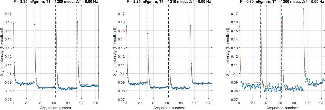
Images were normalized by an independent measurement of M0. Control and label signal was calculated for six myocardial segments, based on AHA’s model, by spatial averaging [8]. The quantification of blood flow for each segment is performed by dictionary matching with a 3-parameter dictionary chosen from sensitivity analysis (See Figure 5).

Results

Figure 2 demonstrates the equivalence between the pulsed ASL signals obtained with Buxton’s general kinetic model [6] and with the modified propagation approach.

Figure 3 shows the bias and variance of dictionary matching for 1- and 3-parameter models. The variance of blood flow for the 3-parameter models (columns 3-4) were comparable with that of the 1-parameter model at low SNR (<50). The 3-parameter model (F,T1,∆f) was chosen as the model of minimum order since the variance of each parameter decreases rapidly with diminishing bias in all modeled parameters as SNR increases.

Figure 5 shows representative examples of dictionary matching for regional SPASL signals. The mean myocardial blood flow in 5 datasets is 2.44 ± 1.01 ml/g/min, which is consistent across animals (2.8, 1.53, 1.54, 2.34, and 3.98). All three examples give reasonable F values.

Discussion

One segment was rejected due to bSSFP banding artifacts. Poor fits were visually observed in 4 out of 29 segments in 5 datasets. These segments corresponded with areas of high off-resonance and/or imaging artifacts. This model also didn’t account for magnetization transfer effects that may have led to over/under estimation of modeled parameters.

Conclusion

Future work will incorporate magnetization transfer effects using the Bloch-McConnell equations and validate dictionary-based quantification against micro-spheres in animal studies.

Acknowledgements

Grant Support: NIH R01-HL130494

References

1. Capron T, Troalen T, Robert B, Jacquier A, Bernard M, Kober F. Myocardial perfusion assessment in humans using steady-pulsed arterial spin labeling. Magn Reson Med. 2015;74:990–998.

2. Xu J, Qin Q, Wu D, et al. Steady pulsed imaging and labeling scheme for noninvasive perfusion imaging. Magn Reson Med. 2016;75:238‐248.

3. Detre JA, Leigh JS, Williams DS, Koretsky AL. Perfusion imaging. Magn Reson Med 1992; 23:37-45.

4. Hargreaves BA, Vasanawala SS, Pauly JM, Nishimura DG. Characterization and reduction of the transient response in steady- state MR imaging. Magn Reson Med 2001;46:149–158.

5. Scheffler K. A pictorial description of steady-states in rapid magnetic resonance imaging. Concepts Magn Reson 1999;11:291–304.

6. Buxton RB, Frank LR, Wong EC, Siewert B, Warach S, Edelman RR. A general kinetic model for quantitative perfusion imaging with arterial spin labeling. Magn Reson Med 1998;40:383–396.

7. Javed A, Jao TR, Nayak KS. Motion correction facilitates the automation of cardiac ASL perfusion imaging. J Cardiovasc Magn Reson 2015;17(Suppl 1):P51.

8. Jao T, Zun Z, Varadarajan P, Pai R, Nayak K. Mapping of myocardial ASL perfusion and perfusion reserve data. In Proceedings of the 19th Scientific Sessions of ISMRM, Montreal, Canada, 2011. p. 1339

Figures

Figure 1: Illustration of the Bloch Simulation. Shown is a balanced SSFP acquisition with variable FA, TR, and TE. Using the hard-pulse approximation, the amount of labeled blood over a time interval is estimated by multiplying the ASL bolus signal $$$s(t)$$$ at the start time $$$t_{i}$$$ of the $$$i^{th}$$$ time interval with the duration $\tau$ of the interval. Inflowing blood is modeled as an impulse and is added to the longitudinal magnetization prior to RF excitation. In experiments, we used a fixed FA/TR/TE bSSFP acquisition, but the simulation method is flexible.

Figure 2. Simulated pulsed ASL signal obtained with (a) the standard model and with (b) the proposed numerical approach. Simulation parameters are M₀= 1, λ = 1, α₀ = 2 (inversion), f = 0.8 ml/g/min, Δt = 0.5 s, τ = 1.0 s, T₁ = 1.0 s, and T₂ = infinite s. Different sampling rates are used to emphasize the detrimental effects of a large sampling interval on the accuracy of the ASL difference signal (c vs. d). In case of TR < 6ms, this difference was always < 0.002%.

Figure 3. Bias and variance plot for (column 1) a 1-parameter model and (columns 2-4) 3-parameter models (See methods). The colored solid line and shaded area represents an estimated mean value and ±SD of sensitivity analysis, respectively. The black solid line is the ground truth and the dotted line indicates the range of a parameter used in a dictionary. Parameters are indicated by different colors. The bias is the discrepancy between colored and black lines. For non-modeled parameters in each model, ground truth values were used (transit delay = 300 ms, T1=1200 ms, T2 = 50 ms, ∆f = 0Hz).

Figure 4. Comparison of bias of (column 1) the 1-parameter model (F) and (column 2) 3-parameter model (F, T1, ∆f). (row 1) Bias plot for (row 1) blood flow of 1 ml/g/min and for (row 2) blood flow of 4 ml/g/min. The range of error in T1 and off-resonance was [-50:1.5:50 ms] and [-50:1.5:50 Hz], respectively. Bias analysis was performed at an SNR of 50 with 1000 realizations.

Figure 5. Representative examples of dictionary matching on regional signals. (left and middle) Two examples of a “good fit”. (right) One example of a “poor fit”. Signal intensities of a segmental signal are blue dots and the matched dictionary entries are red lines. The vertical dotted line indicates a time interval between series measurement for full relaxation of magnetization. The estimated parameters (F, T1, ∆f) are indicated on top of each figure. The strength of the proposed approach is demonstrated in its ability to generate an up-rise trend towards the end of first control series for a fixed blood flow.

Proc. Intl. Soc. Mag. Reson. Med. 27 (2019)

2191