2133
Cardiac short-axis slice range classification via transfer learning: Evaluation of seven popular deep CNNs1Sogang University, Seoul, Korea, Republic of, 2Samsung Medical Center, Sungkyunkwan Univ., Seoul, Korea, Republic of
Synopsis
In cardiac MRI, left ventricle (LV) segmentation typically follows the identification of a short-axis slice range, which may require a manual procedure. The standard cardiac image processing guidelines indicate the importance of correct identification of the slice range. In this study, we investigate the feasibility of deep learning in automatically classifying the slice range. Images were classified into one of three categories: out-of-apical (OAP), apical-to-basal (IN), and out-of-basal (OBS). We developed our in-house user interface to label image slices into one of the three categories for learning. We evaluated the performance of the models, fine-tuned from seven popular deep CNNs.
Introduction
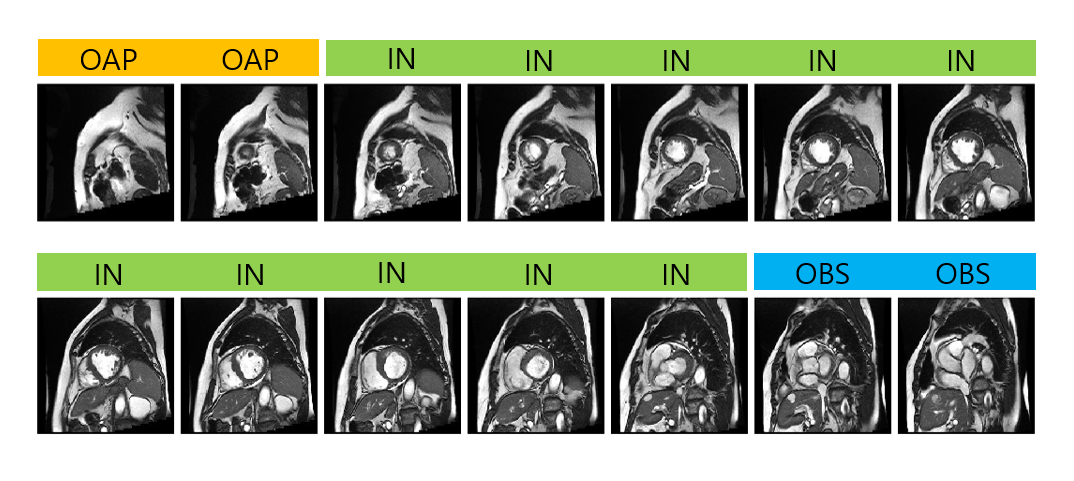
With the recent advances in deep convolutional neural networks (CNNs), there is a growing interest in applying this technology to medical image analysis. In cardiac MRI, deep CNNs are applied to left ventricle (LV), right ventricle (RV), and myocardial segmentation for automatic quantification of ejection fraction and myocardial mass. The segmentation step typically follows the identification of a short-axis slice range, which may require a manual procedure. Figure 1 illustrates the need to automate slice range classification. The standard guidelines provided in Schulz-Menger et al.1 suggest correct identification of slice range for diastole and systole for LV systolic, diastolic volume as well as LV mass. This study aims to develop a deep CNN that can accurately and automatically classify the slice range using transfer learning of existing deep CNNs, which showed remarkable recognition performance in ImageNet.Methods
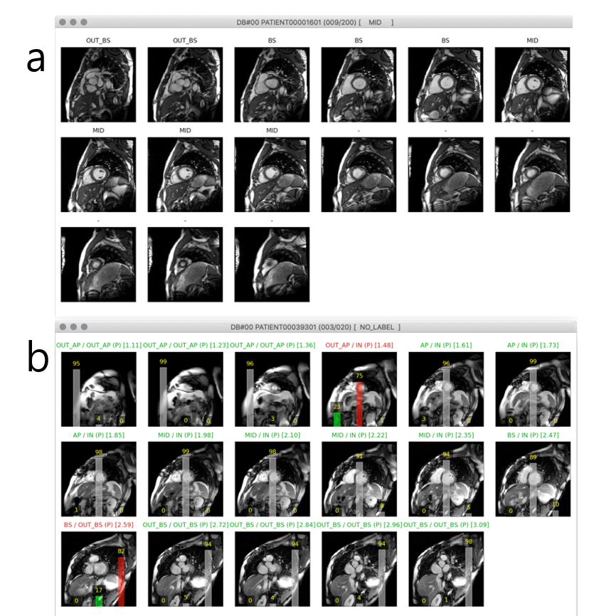
Cardiac short axis cine data available from the LV Segmentation Challenge2 were used for slice range classification. In our study, data consisted of 120 subjects, 80 in the training set / 20 in the validation set / 20 in the test set. We developed a custom user interface in Python 3.6 for image labeling in a diastolic and a systolic frame for all subjects. Figure 2 shows screenshots of the user interface for labeling and for prediction. For labeling, the user interacts with the layout to classify each short-axis slice into one of the three categories: out-of-apical (OAP), apical-to-basal (IN), out-of-basal (OBS).
The number of images prior to data augmentation was (training, testing) = (386, 70) for OAP, (1808, 402) for IN, and (328, 54) for OBS. We used data augmentation by applying random rotation within the range of -40 to 40 degrees and generated five augmented variants of each image. To overcome the imbalance between the number of images in the OAP, OBS, and IN categories, we augmented the number of images from the OAP and OBS categories during training.
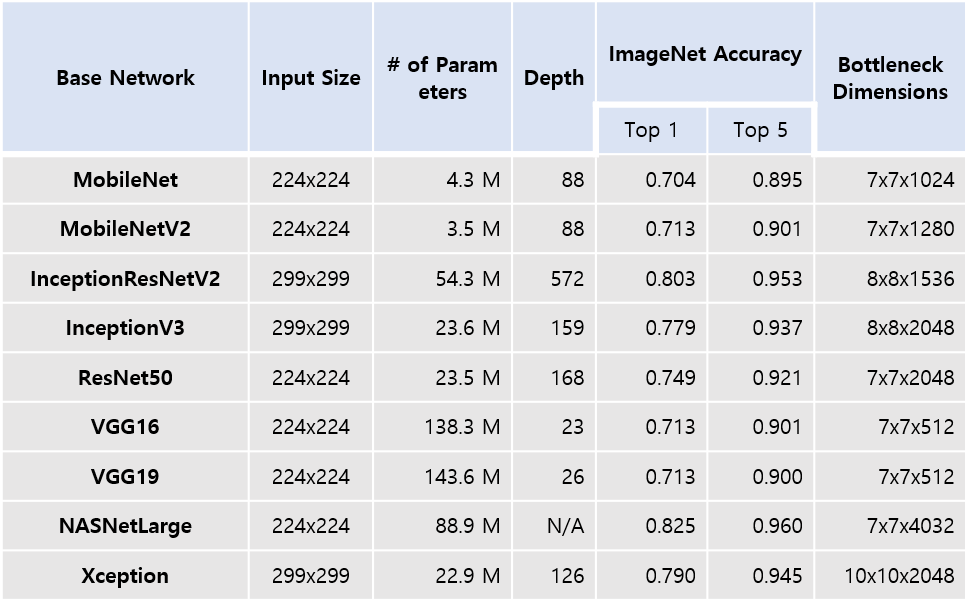
Nine popular deep CNN models were considered for transfer learning. Table 1 lists the models, their capacities, and ImageNet accuracy scores. The model parameters of the layers were reused, except those for fully connected (FC) layers. The last layer's output data, just prior to the first FC layer (a.k.a. bottlenecks), were generated. The training and validation were performed on a single GPU (NVIDIA GeForce 1070, 8GB memory) in Keras. The NASNet and Xception models have relatively large bottleneck dimensions and resulted in GPU memory error during fine-tuning. Hence, only the remaining seven models were considered for model development and validation. These bottleneck data were flattened into a 1D vector, which became the input to an FC layer. The FC layer produced 256 units as output followed by another FC layer to produce probability scores for the three categories via softmax.
Results
Training, validation, and testing of all seven models took approximately 12 hours on a single GPU (NVIDIA GeForce 1070, 8GB memory) when three different learning rates, five-fold cross validation, and 50 epochs were used for learning.
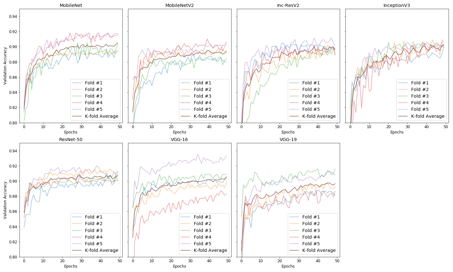
Figure 3 compares epochs vs. validation accuracy plots of five folds for the seven models. It indicates that variation in validation accuracy among the five folds was low for ResNet-50 and high for VGG-16. For InceptionV3, validation accuracy increased slowly with respect to epochs.
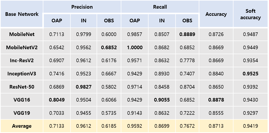
Table 2 compares precision, recall, accuracy, and soft accuracy results among the seven models in testing. All models produced accuracy > 0.85 and soft accuracy > 0.92. Precision for outer slices (i.e., OAP, OBS) was low, ranging 0.57 – 0.80. Recall for outer slices (i.e., OAP, OBS) was 0.68 – 1.0.
Discussion
In this study, we applied the concept of transfer learning to the problem of automatic slice range classification in cardiac short axis images. The precision, recall, and accuracy of the seven models were compared. Although it is difficult to conclude which models show the best performance, even “light” models such as MobileNet and MobileNetV2 appear feasible choices in the classification problem.
Our approach is based on the classification of a single slice image, but it may be more appropriate if one can model the dependency of contiguous short-axis slices from apex to base. Possibly, one can consider modeling a recurrent neural network which takes multiple contiguous short-axis slices as input and corresponding slice labels as output.
Conclusion
The models fine-tuned from seven popular deep CNNs produced high accuracy overall in the classification of three different categories (OAP, IN, OBS). Further studies are necessary in order to improve precision and recall in OAP and OBS categories.Acknowledgements
This work was supported by the Basic Science Research Program through the National Research Foundation of Korea (NRF-2018 R1D1A1B07042692).References
1. Schulz-Menger, Jeanette, et al. "Standardized image interpretation and post processing in cardiovascular magnetic resonance: Society for Cardiovascular Magnetic Resonance (SCMR) board of trustees task force on standardized post processing." Journal of Cardiovascular Magnetic Resonance15.1 (2013): 35.
2. Fonseca, Carissa G., et al. "The Cardiac Atlas Project—an imaging database for computational modeling and statistical atlases of the heart." Bioinformatics 27.16 (2011): 2288-2295.
Figures