2132

Fully Automated Cardiac Bounding Box Detection for Localized Higher-Order Shimming Using Deep Learning

Asha K. Kumara Swamy^1,2, Chandrashekar M. Patil², Punith B. Venkategowda¹, Vikram Nagalli¹, Michael Wangler³, Michaela Schmidt⁴, and Jens Wetzl⁴

¹Siemens Healthcare Private Ltd., Bangalore, India, ²Vidya Vardhaka College of Engineering, Mysore, India, ³Syngo, Siemens Healthcare GmbH, Forchheim, Germany, ⁴Magnetic Resonance, Siemens Healthcare GmbH, Erlangen, Germany

Synopsis

Localized higher-order shimming is a common method for improving image quality in phase sensitive sequences used in cardiac imaging, but requires the manual placement of a three-dimensional bounding box around the heart in which the localized shimming is performed. We present an automated method for detecting such a bounding box from the localizer images using Deep Learning. Two-dimensional bounding boxes are first detected in each localizer slice and then combined to one three-dimensional bounding box. We compare two approaches, either training individual models for each localizer orientation or a joint model for all orientations.

Introduction

In cardiac imaging, many sequences are phase sensitive and suffer from B₀ inhomogeneities, e.g. balanced steady-state free precession (bSSFP), especially at higher field strengths. A common measure is localized higher-order shimming, which requires a bounding box placed tightly around the heart to improve homogeneity within this bounding box. In current clinical practice, this is usually performed manually by the operator. In this abstract, automated bounding box detection for shimming based on a deep learning approach is investigated in order to save operator time as well as increase standardization and repeatability of cardiac scanning protocols.

Methods

Cardiac localizer scans were acquired in 160 healthy volunteers on different $$$1.5\,\textrm{T}$$$ and $$$3\,\textrm{T}$$$ clinical MRI scanners (MAGNETOM Aera, Skyra, Sola, Vida; Siemens Healthcare, Erlangen, Germany) using a bSSFP sequence. Each localizer scan included between 3 and 7 slices in coronal, sagittal and axial orientation to cover the heart, with a fixed $$$(400\,\textrm{mm})^2$$$ field-of-view at a resolution of $$$(1.56\,\textrm{mm})^2$$$. The dataset was divided into 80% training data, 10% validation data and 10% test data. Data augmentation by rotation, scaling and translation was performed to increase the size of the training set.

Annotation: In sagittal orientation, the superior limit of the bounding box was chosen to include ventricles and atria, but without including the aortic arch. In sagittal and axial orientations, the posterior limit was chosen to include the descending aorta, if it was visible. In coronal orientation, the superior limit of the bounding box was chosen to include ventricles and atria up to the pulmonary artery, but without including the aortic arch. If the heart is not clearly visible, the slice is rejected for bounding box detection.

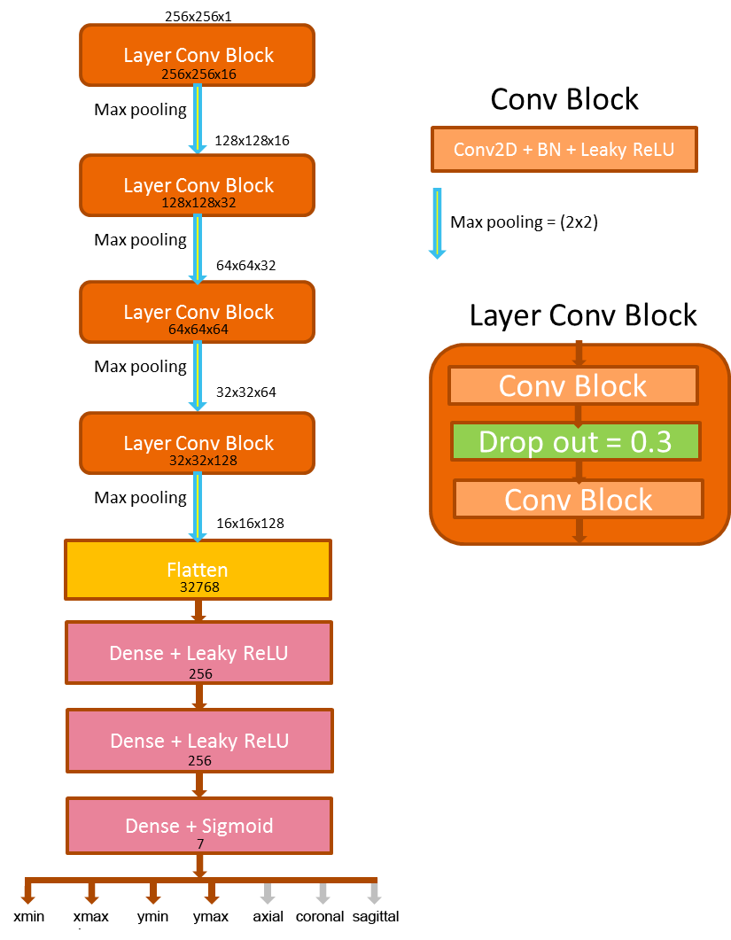
Model Architecture: We compare two prototype approaches in this abstract: The first is to train orientation-dependent networks separately for sagittal, coronal and axial images. The second is to train one combined model for all orientations. To regularize the second network, a multi-task learning approach is chosen whereby the network has to classify the input image orientation as well as the heart bounding box. Both approaches localize the heart in each 2D image slice separately. The combination to a 3D bounding box is performed as a post processing step afterwards¹. Details of the network structure are given in Figure 1. The output layer consists of 4 nodes (x_min, x_max, y_min, y_max) in the first approach and 7 nodes (x_min, x_max, y_min, y_max, axial, coronal, sagittal) in the second approach. After 2D bounding box detection on each individual slice, a random sample consensus² algorithm was performed to remove detection outliers and combine the 2D bounding boxes from the consensus set to a 3D bounding box covering the heart.

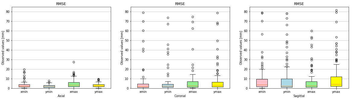
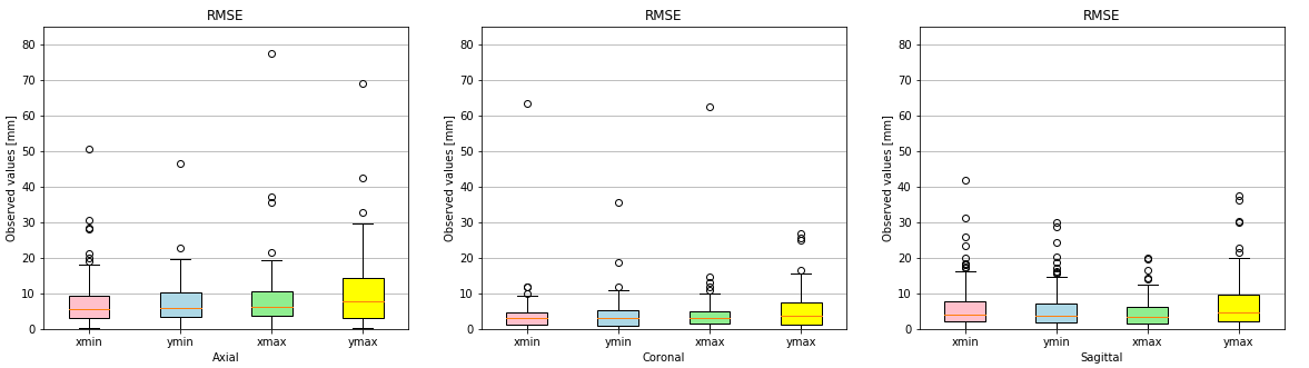
Evaluation: We computed the root-mean-squared error (RMSE) between ground truth annotations and detected results on the testing set for each of the four bounding box coordinates xmin, xmax, ymin and ymax. For the orientation-independent model, we additionally computed sensitivity and specificity of the orientation classification.

Results

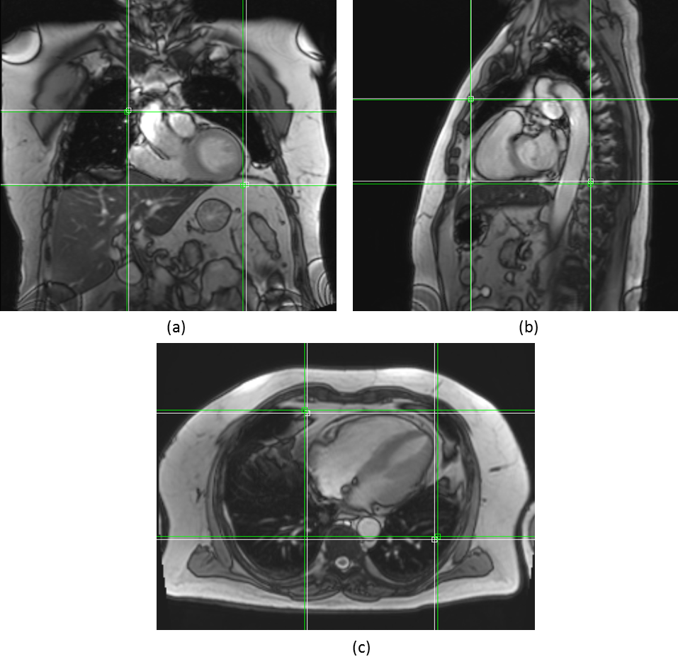
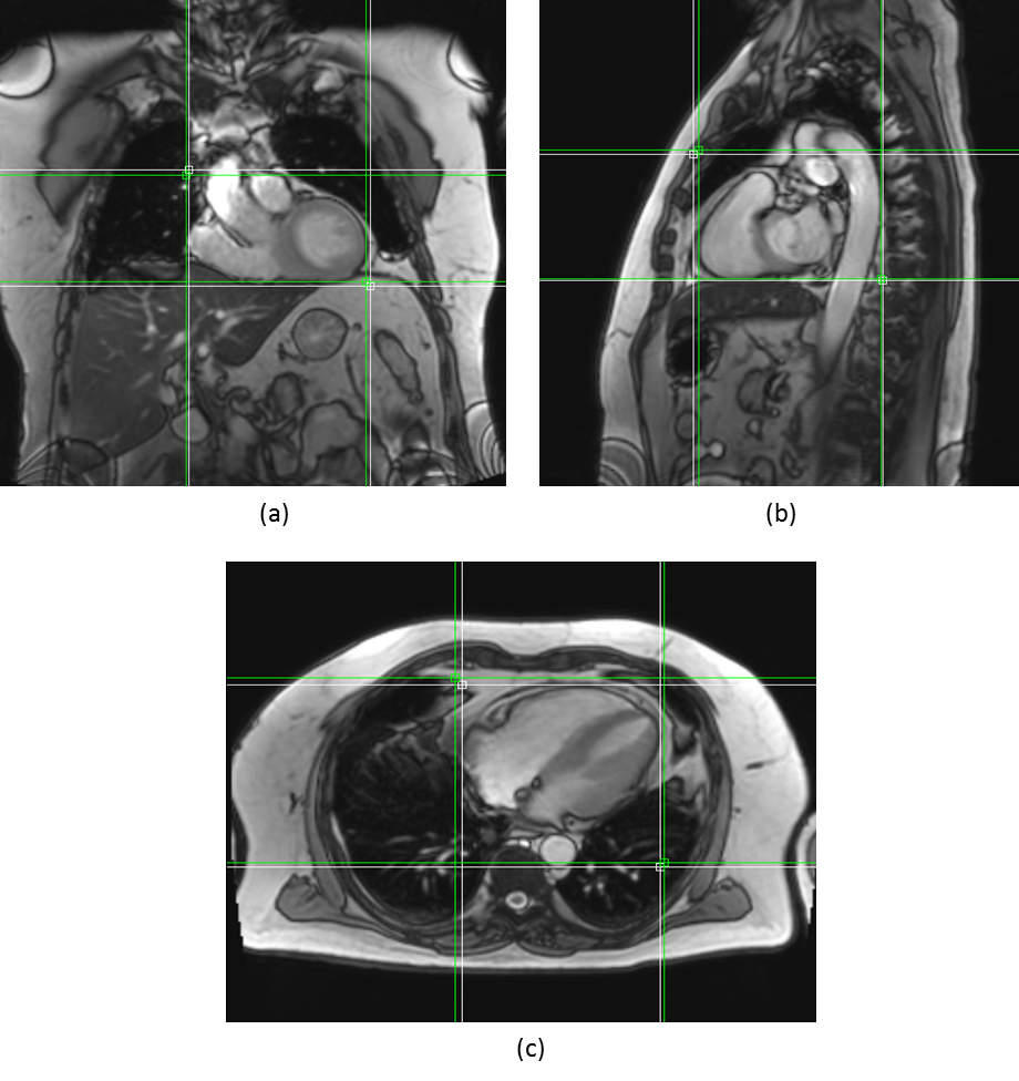
Figures 2 and 3 qualitatively show ground truth annotations and detected bounding boxes for a representative case from the test set based on the orientation-dependent and orientation-independent models, respectively. Figures 4 and 5 show box plots of RMSE values on the entire testing set for each model. Sensitivity and specificity for the orientation classification were 100%, all image orientations were classified correctly.

Discussion

The qualitative results in Figures 2 and 3 show a good match between ground truth annotations and detected bounding boxes for both models. As the acquired data contained more slices in axial orientation than coronal and sagittal ones, the orientation-dependent axial model shows better generalization with a mean RMSE of $$$3.6\,\textrm{mm}$$$ compared to $$$9.8\,\textrm{mm}$$$/$$$8.7\,\textrm{mm}$$$ for sagittal/axial orientation. The coronal and sagittal models show a higher number of outliers. Training a combined orientation-independent model improves the RMSE and reduces the number of outliers for coronal and sagittal models, lowering the 90^th percentile from $$$28\,\textrm{mm}$$$/$$$22\,\textrm{mm}$$$ to $$$13\,\textrm{mm}$$$/$$$9\,\textrm{mm}$$$, respectively. However, it performs slightly worse for the axial orientation. Increasing the model complexity of the orientation-independent models might improve performance for axial slices.

Conclusion

We presented a new approach for automated placement of a shimming volume. While the orientation-dependent approach shows more accurate results for larger numbers of training data, the orientation-independent approach can be used to get more consistent results for smaller training sets.

Acknowledgements

No acknowledgement found.

References

B. de Vos et al. ConvNet-based localization of anatomical structures in 3D medical images. IEEE Trans. Med. Imaging 36(7):1470–1481, 2017.
T. Strutz. Data Fitting and Uncertainty, Springer Vieweg, 2016.
A. L. Maas et al. Rectifier Nonlinearities Improve Neural Network Acoustic Models. Proceedings of the 30th International Conference on Machine Learning, Atlanta, Georgia, USA, 2013.
X. Glorot et al. Understanding the difficulty of training deep feedforward neural networks. International Conference on Artificial Intelligence and Statistics, pp. 249–256, 2010.

Figures

Figure 1. The cardiac bounding box detection consists of eight convolution layers of kernel size 3x3 and four max pooling layers of kernel size 2x2. Each convolution operation is followed by batch normalization and Leaky ReLU³. Spatial dropouts with a dropout rate of 0.3 are introduced between consecutive convolutions. After convolution, a flattening operation is followed by three dense layers, two with Leaky ReLU activations and one with a sigmoid activation. The orientation-independent model has seven output nodes (x_min, x_max, y_min, y_max, axial, coronal, sagittal) while the orientation-dependent model lacks the last three. The Xavier normal initializer⁴ is used for weight initialization.

Figure 2. Orientation-dependent model: Representative results of bounding boxes detected in coronal (a), sagittal (b) and axial (c) orientations, represented by the green lines, compared to the ground truth annotations, represented by the white lines.

Figure 3. Orientation-independent model: Representative results of bounding boxes detected for the same images as figure 2 using the orientation-independent model.

Figure 4. Box plots of the RMSE between ground truth and deep learning results of the test set based on the orientation-dependent model for axial (left), coronal (middle) and sagittal orientations (right).

Figure 5. Box plots of the RMSE between ground truth and deep learning results of the test set based on the orientation-independent model for axial (left), coronal (middle) and sagittal orientations (right).

Proc. Intl. Soc. Mag. Reson. Med. 27 (2019)

2132