Synopsis

To investigate abnormal hemodynamics in pulsatile tinnitus patients in vivo, we use 4DMR. We also use computational fluid dynamics (CFD) to overcome 4DMR’s limited spatial and temporal resolution. To ensure the simulation actually reflects in vivo blood flow, we systematically adjust the simulation boundary conditions to match the CFD and 4DMR data. This requires downsampling CFD data to 4DMR resolution and a quantitative voxel-wise comparison. Our results suggest 4DMR underestimates velocities in vivo due to its resolution. This effect is confirmed by phantom 4DMR data taken at multiple resolutions.

Introduction

Methods

Patient data acquisition and processing

A patient with PT suspected to originate from a transverse sinus diverticulum was imaged on a 3T Siemens scanner using 4DMR (at 1.1 x 1.1 x 1.4 mm³ resolution) and CE-MRA (at 0.5 x 0.5 x 0.5 mm³ resolution) to obtain the in vivo velocity field and geometry. The 4DMR data was processed using in-house Python tools. As a starting point, the blood flow was measured from 4DMR and used as a boundary inlet condition for the CFD simulation.

CFD downsampling and readjustment

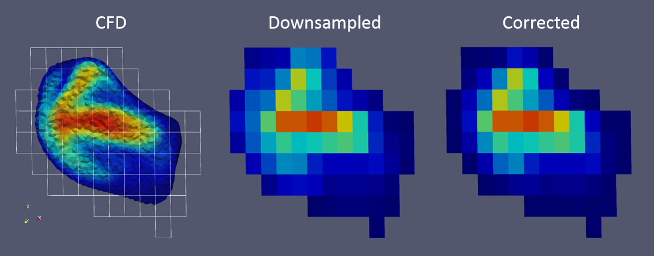
To quantitatively compare CFD and 4DMR, the CFD results were first downsampled to MR resolution such that the velocity ($$$a$$$) measured at a voxel is a gaussian distance ($$$w$$$) and volume-weighted ($$$v$$$) average of the neighboring CFD cells found within the voxel’s sampling volume (Figure 1), to mimic MR physics [1][2]:

$$a_{\textrm{voxel}} = \sum_{i=\textrm{cell}}{w_i\cdot v_i\cdot a_i }$$

$$w_i = w(r_i) = \frac{1}{(2πσ^2)^(\frac{3}{2}}e^{-(\frac{r_i}{2σ})^2}$$

At each point, the difference in velocity magnitude was calculated and a local mean error was obtained:

$$\textrm{error} = \textrm{mean of}\frac{\textrm{difference}}{\textrm{MR velocity}} = \frac{ \overline{ v_{CFD,i} - v_{MR,i} } }{ v_{MR,i} } $$

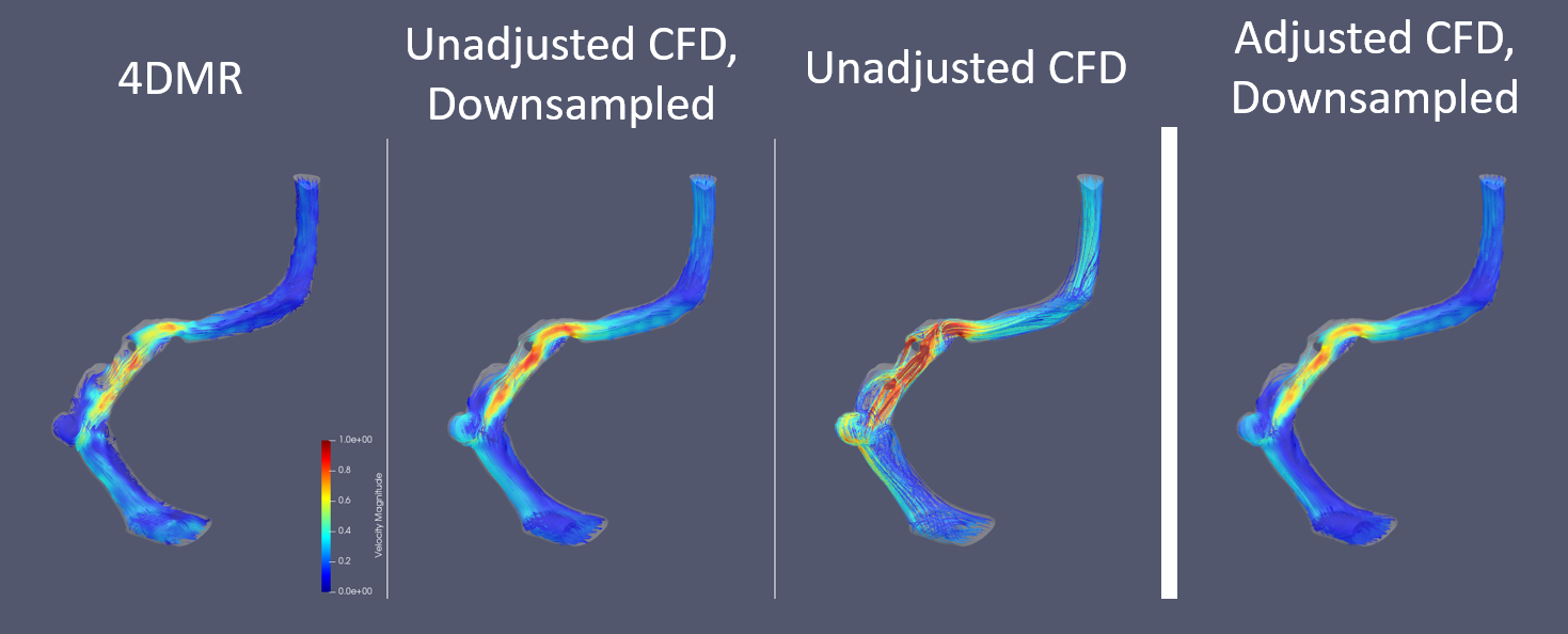
To avoid noise and partial voluming, the error calculation excludes voxels near or at the vessel wall and voxels below a velocity threshold. This error was then used to scale the inlet boundary condition of the next simulation iteration (n+1) as follows (Figure 2):

$$v^{n+1}_{\textrm{inlet}} = \frac{v^{n}_{\textrm{inlet}}}{1 + \textrm{error}}$$

Phantom data acquisition

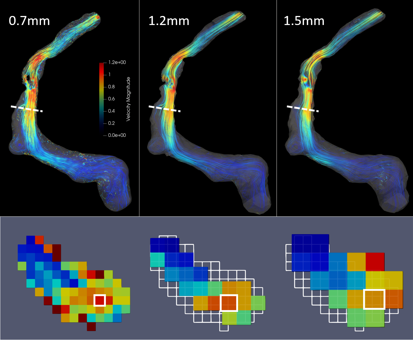
The downsampling process is akin to decreasing image resolution. To confirm its effects on the velocity field experimentally, a silicone phantom created from the patient geometry was imaged to obtain 4DMR results at multiple resolutions: 0.7mm (high), 1.2mm (standard), and 1.5mm (low) isotropic.

Results

The effect of adjusting the CFD results based on the voxelwise comparison between CFD and 4DMR data is provided in Figure 2. Qualitatively, the downsampled and adjusted CFD results are closer to the 4DMR results than the downsampled, unadjusted CFD results. Quantitatively, the mean local velocity error calculated for the unadjusted and adjusted simulations are 0.103 and -0.003, respectively.

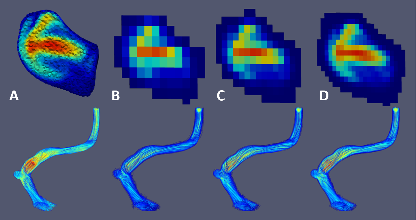
Figure 3 shows streamlines demonstrating the effects of downsampling the CFD results to MR grids of increasing resolution. Downsampling appears to severely affect near-wall velocity values due to voxel contributions from empty space. Inner streamlines are less affected, but velocities in abnormal geometries (diverticulum, arachnoid granulation) are still underestimated. Increasing the resolution retains more of the velocity magnitude and original flow features.

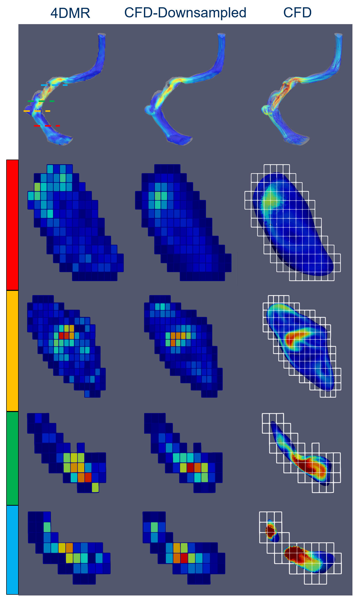
Figure 4 compares the patient 4DMR data to both the original and downsampled CFD results after the CFD has been readjusted. Overall, the velocity field from the CFD simulation appears to be much higher in magnitude than from 4DMR. The velocities are closer after the CFD data is downsampled but many of the detailed flow features may be lost, particularly in thin vessels.

We experimentally confirmed the effects of downsampling by analyzing the 4DMR results in a flow phantom at different resolutions (Figure 5). The overall velocities and local peak velocity drop as the resolution decreases.

Discussion

The downsampling process results in a smoothing effect that underestimates any peak velocities particularly in small vessels and vessel abnormalities. This suggests that in general, 4DMR-derived velocity fields taken at conventional resolutions may underestimate the true in vivo velocity field. Further evidence for this effect is provided from the 4DMR phantom results, which reveal a loss in velocity magnitude as resolution decreases. This is particularly important as research groups increasingly use 4DMR to derive clinically-relevant hemodynamic parameters, such as wall shear stress.

4DMR and CFD can be complementary diagnostic tools: 4DMR is valuable for both validating and adjusting CFD results, while CFD can capture details that may be missed due to noise and low resolution.

Acknowledgements

References

[1] Belen Casas, Jonas Lantz, Petter Dyverfeldt, and Tino Ebbers. 4d flow MRI-Based pressure loss estimation in stenotic flows: Evaluation using numerical simulations: Pressure Loss Estimation in Stenotic Flows Using 4d Flow MRI. Magnetic Resonance in Medicine, pages 1808-21, May 2015.

[2] Haraldsson, H., Kefayati, S., Ahn, S., Dyverfeldt, P., Lantz, J., Karlsson, M., Laub, G., Ebbers, T., Saloner, D., (2018), Assessment of Reynolds stress components and turbulent pressure loss using 4D flow MRI with extended motion encoding, Magnetic Resonance in Medicine, 79(4), 1962-1971. https://doi.org/10.1002/mrm.26853