1958
Accelerated 4D flow MRI using a Low-Rank Tensor reconstruction1Radiology and Nuclear Medicine, Amsterdam UMC, Amsterdam, Netherlands, 2Biomedical Engineering and Physics, Amsterdam UMC, Amsterdam, Netherlands
Synopsis
4D flow MRI provides visualization and quantification of complex blood flow. However, the inherent high dimensionality leads to long acquisition times. In this work, 4D flow MRI was accelerated using the novel Low-Rank Tensor framework. To reduce the amount of unknowns, the 4D flow dataset is approximated by a Tucker decomposition, whose components are obtained from navigator and sparse data with iterative optimization exploiting sparsity after variable k-space undersampling. Using this technique, 4D flow MRI acquisition could be accelerated up to 20 times (flow phantom) and 8 times (in-vivo), while preserving measurement accuracy of high velocity magnitudes and cardiac variability.
Introduction
4D flow MRI provides comprehensive visualization and quantification of blood flow velocity patterns1. However, the inherent high dimensionality leads to long acquisition times. In this work, we aimed to accelerate 4D flow MRI using a recently proposed novel Low-Rank Tensor reconstruction framework2. Low-rank based models have been used before to exploit spatiotemporal correlations, for example to resolve different kinds of body motion from multiple time dimensions3. It is expected such correlations can also be exploited in 4D flow MRI, most notably along the cardiac cycle, to enable acceleration. The approach was validated on a carotid flow phantom with retrospective undersampling and in-vivo prospectively. Reconstruction comparisons were made with fully sampled scans.Methods
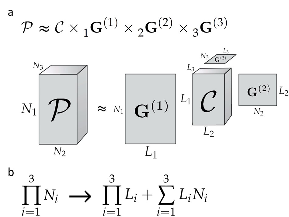
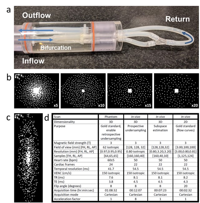
4D flow MRI data is five-dimensional consisting of four spatiotemporal dimensions plus one velocity encoding dimension. In this work, 4-point referenced flow encoding was used to perform 4D flow MRI on a 3T MRI scanner using retrospective gating (Philips Ingenia, Best, The Netherlands). A 4D flow dataset approximation in form of a Tucker decomposition was assumed (Figure 1a). Here, the factor matrix $$$\textbf{G}^{\left(i\right)}$$$ contains the Li principal components in dimension i, and the entries of the core tensor $$$\textbf{C}$$$ show the level of interaction between these components4. When the rank (L1,L2,L3) is relatively low, the number of unknowns is highly decreased (Figure 1b), enabling k-space undersampling. The subspace $$$\left(\left\{\textbf{G}^{\left(i\right)}\right\}_{i=2}^3\right)$$$ was estimated from navigator data fully sampled along dimension i. $$$\textbf{G}^{\left(1\right)}$$$ and $$$\textbf{C}$$$ were found from a sparse dataset by iterative optimization with sparsity constraints. Our novel approach was tested on a pulsatile flow phantom (Figure 2a) mimicking a carotid bifurcation. A fully sampled 4D flow MRI scan was performed as a gold standard reference, using a 32-channel head coil. Subsequently, to simulate accelerated scans, this fully sampled scan was retrospectively undersampled using variable density patterns (Figure 2b), incoherent over time and velocity encoding directions. Acceleration factors of R=5,10,15 and 20 were simulated. Regularization parameters were tuned by minimizing the velocity difference sum-of-squares between reconstruction and gold standard over the whole dataset. Flow curves, and through-plane velocity profiles and color maps were calculated from ROIs drawn in the same slices (GTFlow, Gyrotools, Zurich, Switzerland). The technique was applied in-vivo, on a healthy volunteer. This was prospectively undersampled with incoherent undersampling over time and velocity encoding directions using the in-house developed PROUD software patch5,6, with R=8 (Figure 2c) and an 8-channel neck coil. Due to the current inability to acquire navigator and sparse data prospectively simultaneously, an additional fully sampled but low-resolution subspace estimation scan was performed. To assess image quality, a velocity vector profile was acquired using GTFlow. Flow curves were acquired and compared with flow curves obtained from a fully sampled 2D scan at identical location. Regularization parameter choice was based on the phantom experiment values. Additional scan parameters of all scans are given in Figure 2d. Reconstructions were performed slice-by-slice in frequency encoding direction, giving separate Tucker decompositions for each frequency encoding slice.
Results
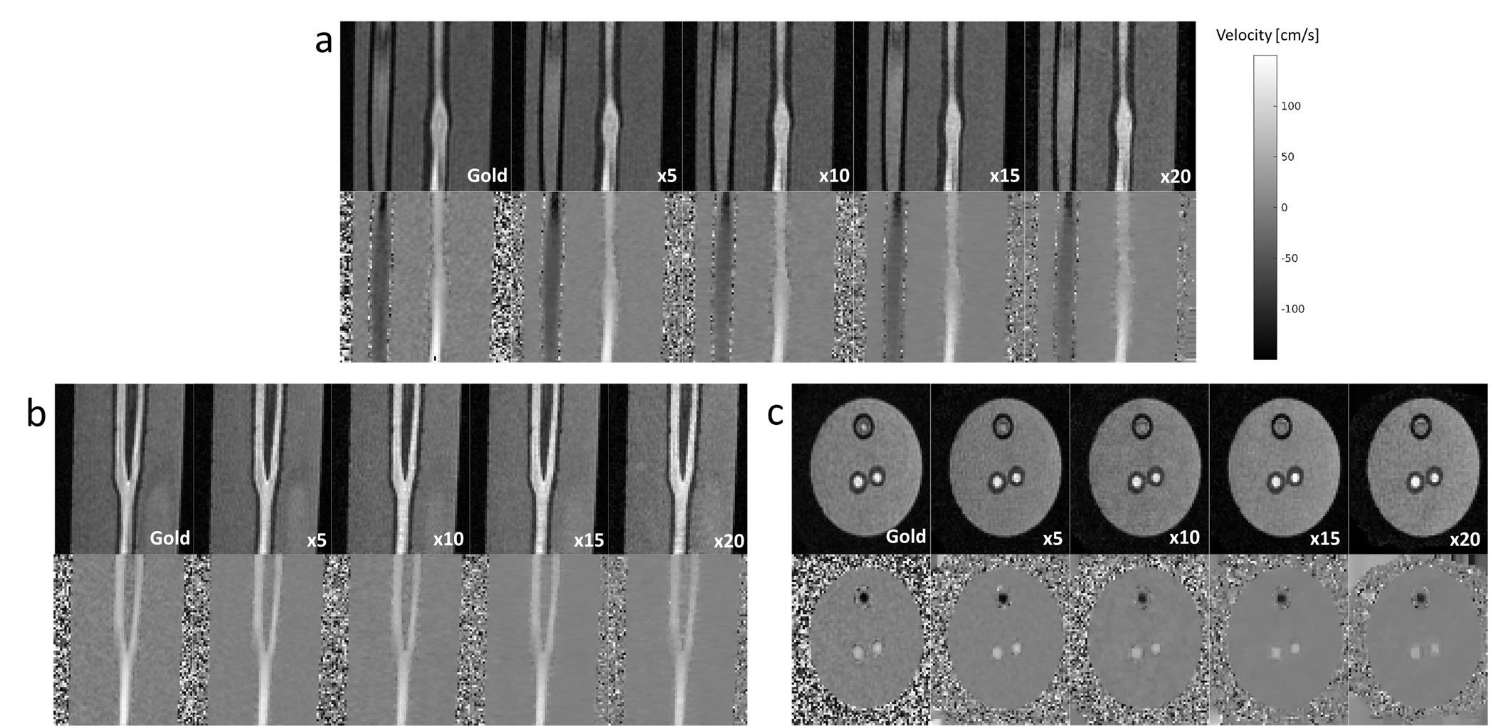
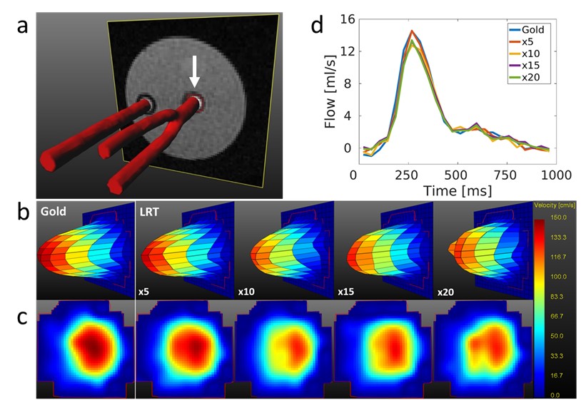
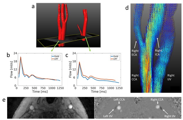
For the phantom, Figure 3 shows very good agreement of magnitude and velocity images with the gold standard, with a slight contrast reduction at higher R. The through-plane peak velocity profiles and color maps in Figure 4b,c show good and fair preservation of velocity magnitude and spatial distribution, respectively, for increasing acceleration. The flow curves in Figure 4d confirm this good performance in the same slice, with similar patterns for all R. In-vivo, the flow curves in Figure 5b,c show a high consistency between the accelerated 4D flow MRI and 2D reference scans. In Figure 5d, LRT shows the ability to produce reliable velocity vector profiles at R=8, both in the carotid bifurcation and the internal jugular vein. Figure 5e demonstrates the ability to reconstruct velocity images in-vivo. Also, for both experiments, a substantial denoising effect is visible.Discussion
The LRT approach is able to reconstruct flow velocities from up to x20 undersampled phantom data, both at peak flow and along the cardiac cycle. The in-vivo scan shows the same for R=8. Moreover, a reduction of (high-rank) noise is visible in both experiments. Reconstruction of lower in-plane velocities is currently suboptimal. Possible solutions to this issue could be removing non-flowing background voxels prior to subspace estimation, employing for example the Hadamard transform7, and to increase rank values.Conclusion
We were able to apply the LRT framework to 4D flow MRI. In general, high velocities are well reconstructed even for high acceleration numbers. Additional consideration is recommended for complex flow and low velocities.Acknowledgements
We thank Maarten Versluis (Philips), Gérard Crelier (Gyrotools) and Martin Bührer (Gyrotools) for their support.References
- Markl M, Frydrychowicz A, Kozerke S, Hope M, Wieben O. 4D flow MRI. J Magn Reson Imaging. 2012;1036:1015-1036. doi:10.1002/jmri.23632.
- He J, Liu Q, Christodoulou AG, Ma C, Lam F, Liang ZP. Accelerated High-Dimensional MR Imaging With Sparse Sampling Using Low-Rank Tensors. IEEE Trans Med Imaging. 2016;35(9):2119-2129. doi:10.1109/TMI.2016.2550204.
- Christodoulou AG, Shaw JL, Nguyen C, Yang Q, Xie Y, Wang N, Li D. Magnetic resonance multitasking for motion-resolved quantitative cardiovascular imaging. Nat Biomed Eng. 2018;2(4):215-226. doi: 10.1038/s41551-018-0217-y.
- Kolda TG, Bader BW. Tensor Decompositions and Applications. SIAM Review. 2009;51(3):455-500. doi: 10.1137/07070111X.
- Peper ES, Gottwald LM, Zhang Q, Coolen BF, van Ooij P, Strijkers GJ, Nederveen AJ. 30 times accelerated 4D flow MRI in the carotids using a Pseudo Spiral Cartesian acquisition and a Total Variation constrained Compressed Sensing reconstruction. Proceedings of the 27rd Annual Meeting ISMRM, 2018;Paris, France.
- Gottwald LM, Peper ES, Zhang Q, Coolen BF, Strijkers GJ, Planken RN, Nederveen AJ, van Ooij P. Pseudo Spiral Compressed Sensing for Aortic 4D flow MRI: a Comparison with k-t Principal Component Analysis. Proceedings of the 27rd Annual Meeting ISMRM, 2018;Paris, France.
- Valvano G, Martini N, Huber A, Santelli C, Binter C, Chiappino D, Landini L, Kozerke S. Accelerating 4D Flow MRI by Exploiting Low-Rank Matrix Structure and Hadamard Sparsity. Magn Reson Med. 2017;78(4):1330-1341. doi: 10.1002/mrm.26508.
Figures