Synopsis

Current software used to process 4D Flow MRI data only allow to quantify a few hemodynamics parameters. Furthermore, the information of these parameters is normally given in a few 2D locations. In this work, we show the development of a novel, free and editable MATLAB toolbox (MathWorks, Natick, MA, USA) called FEMQ-4D that allows the quantification of several hemodynamic parameters in 3D using finite elements (FE) methods. As a complement to this tool, the output of FEMQ-4D, i.e 3D maps of hemodynamic parameters, can be visualized using the open source software PARAVIEW (KitwareInc., Clifton Park, New York, USA).

INTRODUCTION

METHODS AND RESULTS

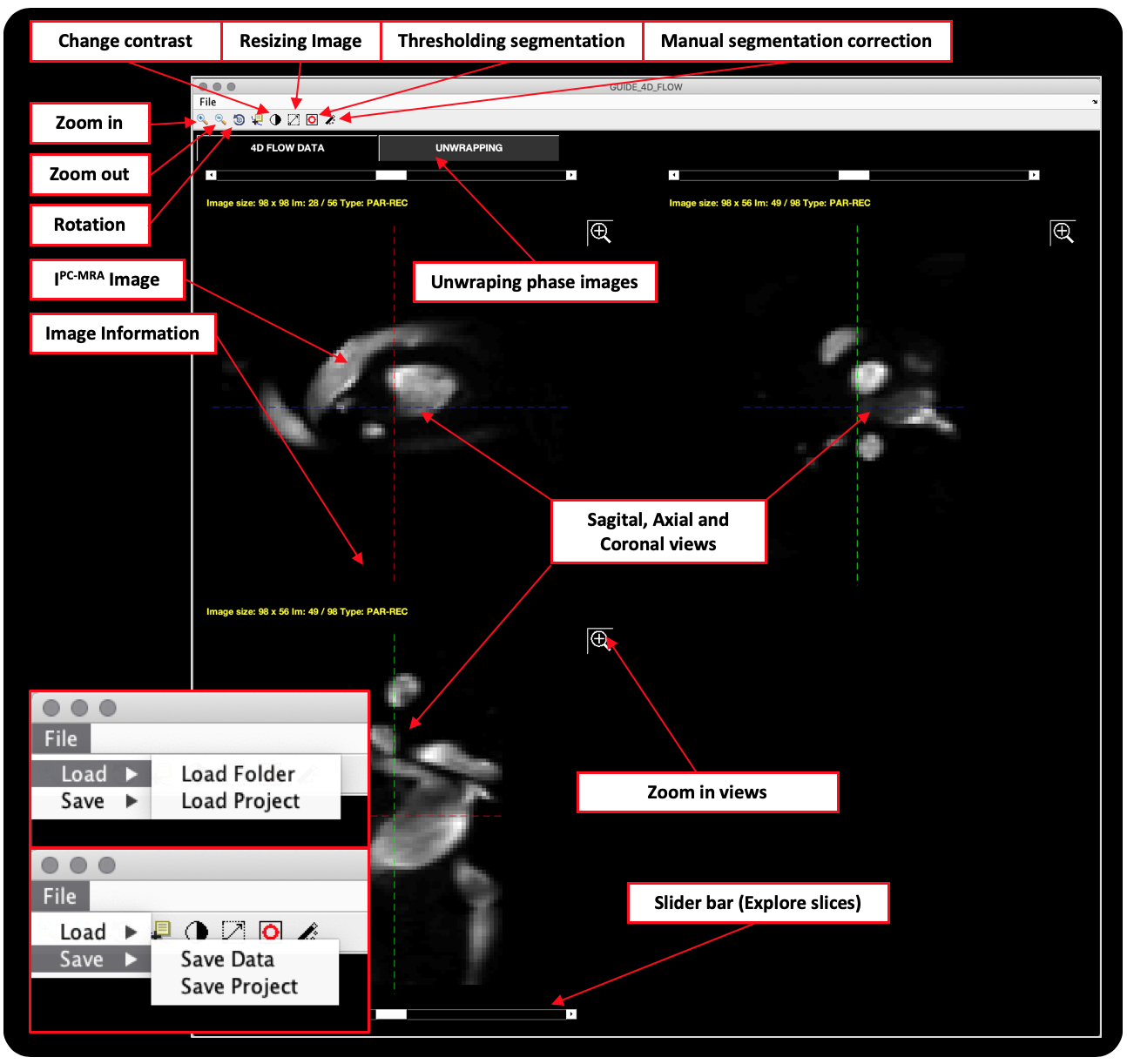
In the Fig.1 we show the main windows of the toolbox. The software is able to read 4D flow data of Philips, Siemens and GE MR scanners. The I^PC-MRA images⁹ are automatically generated when we read data, with exception of GE images, in that we used the complex difference images¹⁰. Additionally, an unwrapping tab¹¹ is included in the toolbox in case of velocity aliasing.

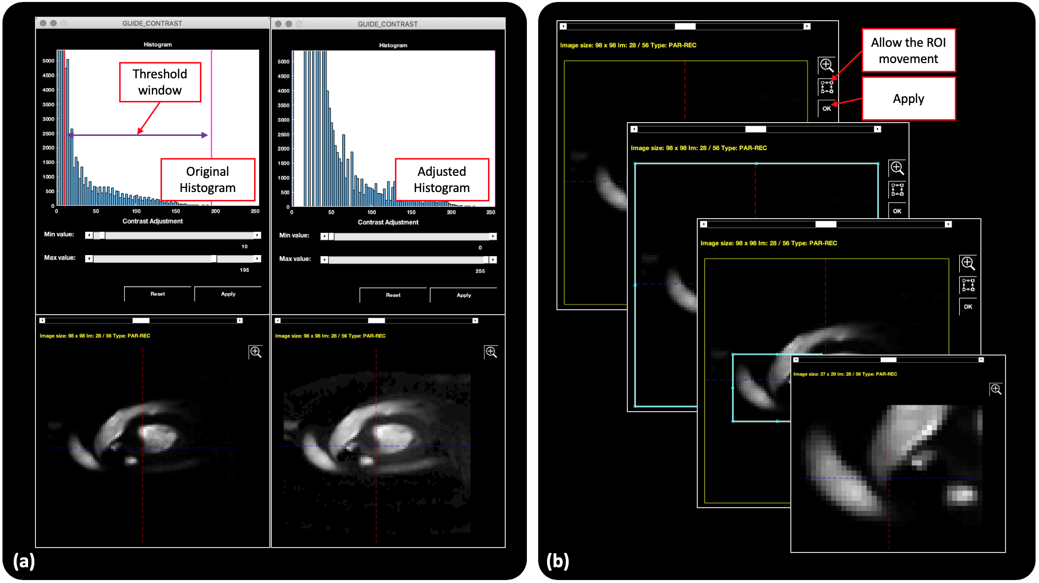
After loading the images, we adjust the contrast of the I^PC-MRA to improve the brightness, expanding the histogram between two selected thresholds Fig.2a. Also, we can resize the image volume by adjusting the contours of the ROI in each view (axial, sagittal or coronal). This tool is very useful to process the GE MR images because these data sets are normally larger than Philips or SIEMENS.

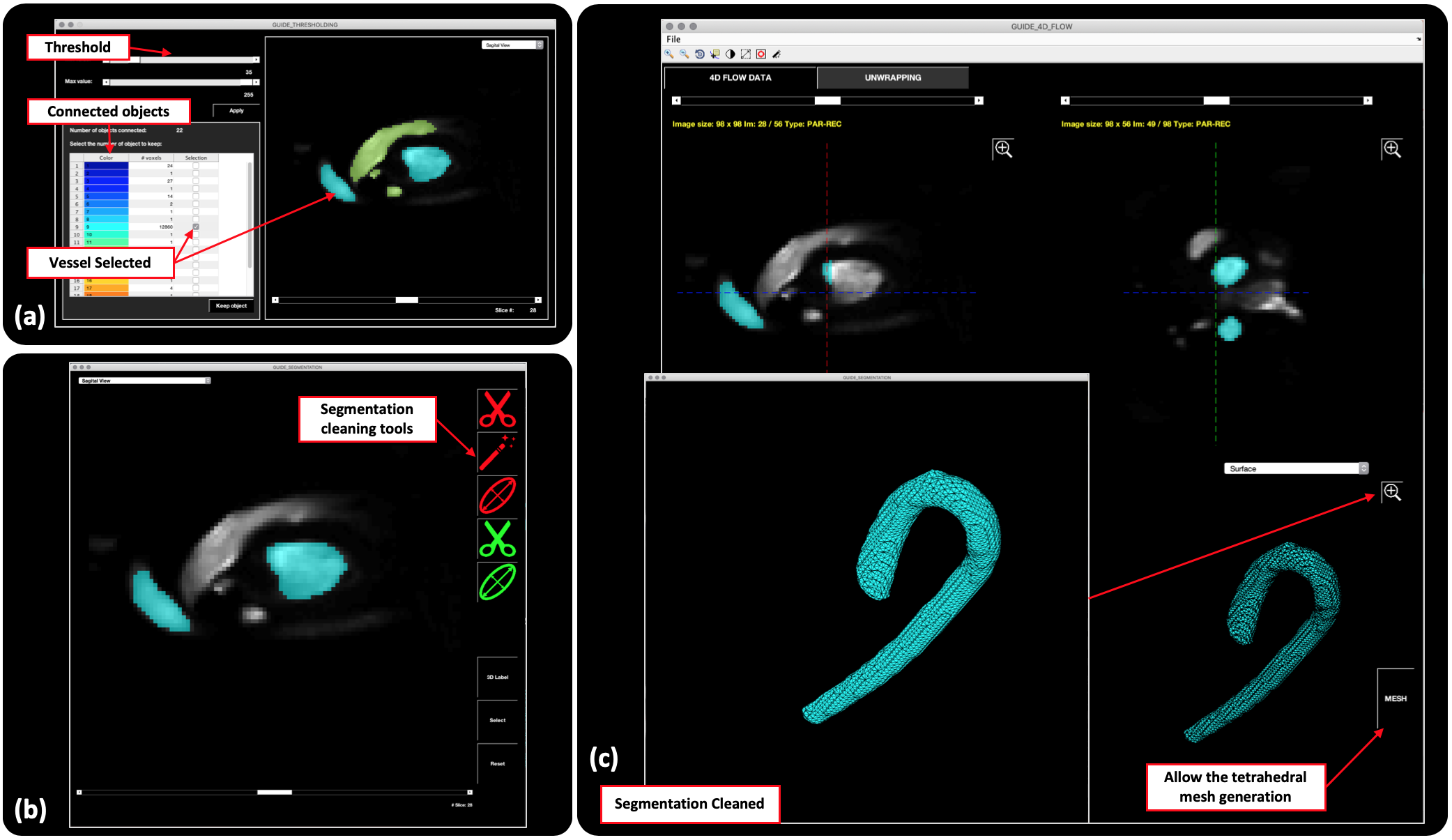
After contrast and resize adjustment, we generate the segmentation of the vessel of interest using a thresholding method and labeling. Each color in Fig3a indicates that one group of voxels are connected between them (we use six neighbor voxels to evaluate the connections), which allows the selection of the vessel that we want to process (aorta). The next step is to clean up the segmentation manually (Fig3b) using the cleaning tools, to add or remove a group of voxels. The final result of this process is shown in Fig3c, which shows the segmentation overlapping the I^PC-MRA images. It is also possible to observe the surface generated by the segmentation. Finally, the result of the clean segmentation allows the use of the MESH button to generate the tetrahedral mesh, which is used to calculate the hemodynamic parameters as described in ^6-8.

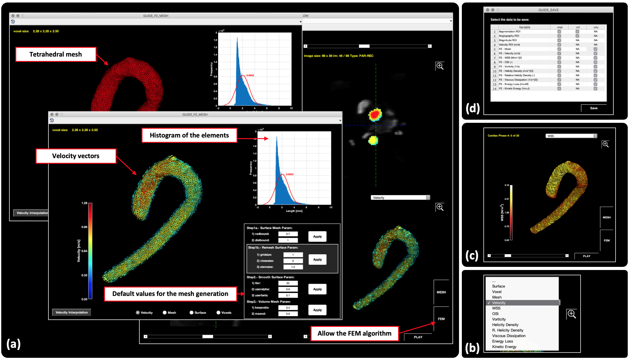
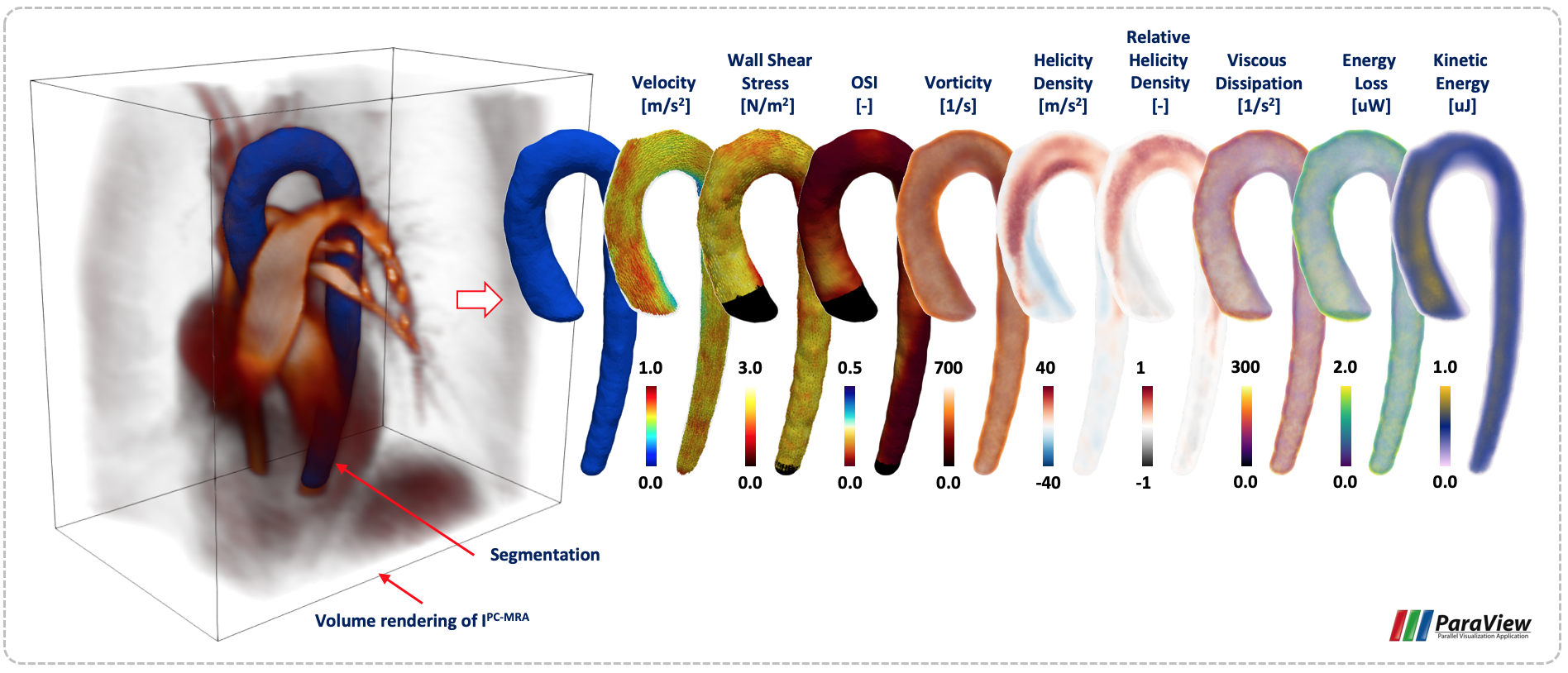
After the mesh creation, we can calculate the hemodynamic parameters using the FEM button. After pressing the FEM button in the popup menu, different hemodynamic parameters are available (Fig.4b). In the current version of the toolbox, we are able to calculate eight different hemodynamic parameters: wall shear stress [N/m²], oscillatory shear index [-], vorticity [1/s], helicity density [m/s²], relative helicity density [-], viscous dissipation [1/s²], energy loss [mW] and kinetic energy [mJ]) from the velocity field obtained by 4D flow data using our FE method^6-8. One example of the hemodynamic parameters calculated with our application (wall shear stress) is shown in the Fig.4c.

Finally, we can save the data in three different formats (Fig.4d), MATLAB files (.mat), PARAVIEW files (.vti and .vtu). The software runs in OSX, LINUX and Windows platform.

Using the PARAVIEW files (.vti and .vtu) previously saved, we can visualize the results of the three-dimensional maps. One example of the three-dimensional maps calculated with our toolbox is shown in Fig.5. It is also possible to visualize the I^PC-MRA image overlapping the segmentation. The estimated time that takes each process are: 1 min for the segmentation and cleaning, 2 min to generate the tetrahedral finite element mesh with the velocity interpolation and 2 min the hemodynamics parameter quantification, save the data in all formats take around 1 min.

DISCUSSION AND CONCLUSION

Acknowledgements

References

1.- GTFlow of Gyrotools (Zurich, Switzerland)

2.- Arterys (San Francisco, CA, USA)

3.- CASS MR Solutions of PIE Medical (Maastricht, Netherlands)

4.- MEDVISO (Lund, Sweden)

5.- CVI of Circle Cardiovascular Imaging (Calgary, AB, Canada)

6.- Sotelo J, Urbina J, Valverde I, et al. Three-dimensional quantification of vorticity and helicity from 3D cine PC-MRI using finite-element interpolations. Magn Reson Med. 2018 Jan;79(1):541-553.

7.- Sotelo J, Urbina J, Valverde I, et al. 3D Quantification of Wall Shear Stress and Oscillatory Shear Index Using a Finite-Element Method in 3D CINE PC-MRI Data of the Thoracic Aorta. IEEE Trans Med Imaging. 2016 Jun;35(6):1475-87

8.- Sotelo J, Dux-Santoy L, Guala A, et al. 3D axial and circumferential wall shear stress from 4D flow MRI data using a finite element method and a laplacian approach. Magn Reson Med. 2018 May;79(5):2816-2823.

9.- Bock J, Frydrychowicz A, Stalder AF, et al. 4D phase contrast MRI at 3 T: effect of standard and blood-pool contrast agents on SNR, PC-MRA, and blood flow visualization.

10.- Johnson KM, Lum DP, Turski PA, et al. Improved 3D phase contrast MRI with off-resonance correcteddual echo VIPR. Magn Reson Med 2009;60:1329–1336.

11.- Loecher M, Schrauben E, Johnson KM, et al. Phase unwrapping in 4D MR flow with a 4D single-step laplacian algorithm. J Magn Reson Imaging. 2016 Apr;43(4):833-42. Magn Reson Med. 2010 Feb;63(2):330-8.