1915
Segmentation of the Cortex and Medulla in Multiparametric Magnetic Resonance Images of the Kidney using K-Means Clustering1MRC Centre for Inflammation Research, University of Edinburgh, Edinburgh Bioquarter, Edinburgh, United Kingdom, 2Liver Unit, Royal Infirmary of Edinburgh, Edinburgh Bioquarter, Edinburgh, United Kingdom, 3BHF Centre for Cardiovascular Science, University of Edinburgh, Edinburgh Bioquarter, Edinburgh, United Kingdom
Synopsis
Magnetic Resonance Imaging (MRI), including T1, T2*, Apparent diffusion coefficient (ADC) and Arterial Spin Labelling (ASL) perfusion, represents a powerful tool for renal investigations. This allows for simultaneous assessment of structure and function in pathologies from Acute Kidney Injury (AKI) to Chronic Kidney Dysfunction (CKD). Differentiation of the medulla and cortex is essential as these tissues have different biomarker distributions. Currently, segmentation of the biomarker histograms is carried out with manual definition of thresholds. Here, we applied K-means clustering to segment the maps and showed that this produced physiologically meaningful results while improving biomarker precision compared with whole kidney regions.
Introduction
Magnetic Resonance Imaging (MRI) represents an ideal method to non-invasively investigate kidney function with biomarkers including MRI relaxation times T1 and T2* plus Apparent Diffusion Coefficient (ADC) and perfusion with Arterial Spin Labelling (ASL). The kidney consists of the outer renal cortex and the inner medulla. In previous studies, segmentation of these anatomical compartments has been achieved in two main ways: splitting of the T1 histogram by identifying two peaks 1 or definition of regions on a structural image 2,3. Although there is good reproducibility in both cases, they require significant user interaction and images registered to a common space. We propose the use of a K-means clustering algorithm to identify the two biomarker distributions within the kidney histogram representing the cortex and medulla values. K-means clustering has been applied to the liver previously for the identification of disease based on the whole image but not to individual parametric maps 4.Methods
Data for segmentation was collected on a 3.0 T Siemens Prisma Scanner (Siemens Healthineers, Erlangen, Germany) with a 16 channel phased array flex coil anterior and 16 channel spine coil posterior.
15 subjects were recruited, 7 with normal kidney function and 8 suffering from renal impairment. The following maps were available for analysis (normal/impaired): T1 11 (5/6), T2* 7 (2/5), ADC 8 (2/6) and ASL 15 (7/8).
All maps were generated using the Siemens console software and then exported offline and processed with MATLAB 2016b (The Mathworks Inc. Natick MA USA). Smoothing with a 3 x 3 matrix was applied and an initial ROI was drawn around the kidney (Fig. 1A). Initial segmentation was carried out that identified background noise in the map to generate a whole kidney ROI that was sub segmented into the cortex and medulla ROIs (Fig. 1B). Clustering was carried out in 3 dimensions; the value of the pixel and its position in X and Y to enforce spatial homogeneity.
The segmentations were checked visually, both that the segmentation was reasonable compared with the known anatomy (Fig. 1) and that the histograms for each segmentation had a single peak (Fig. 2). In the case of segmentation failure an additional region may be included to contain noise or artefacts in the biomarker map. For each individual map the mean (M) biomarker values and standard error in this mean (SEM) were determined for the whole kidney, cortex and medulla regions. Analysis was performed using paired t-tests; a p-value < 0.05 was considered statistically significant.
Results
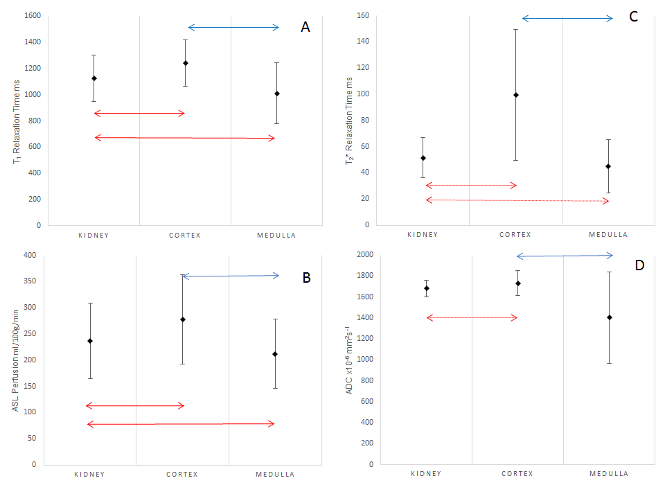
For each biomarker the mean for the subjects with that parameter is shown in Fig. 3 with its SD across the group in the error bars. Significant differences in the means of the regions are indicated with arrows.
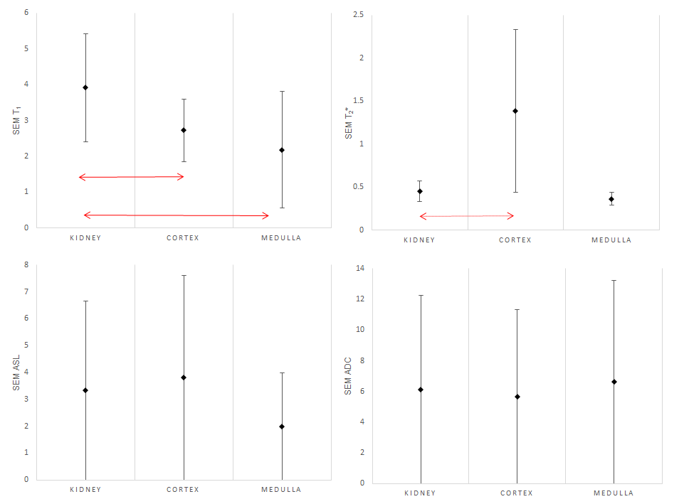
The mean SEM across the subjects with its SD is displayed for each of the biomarkers and regions in Fig. 4. Any significant improvements following segmentation are indicated with arrows.
Discussion
Significant differences between the biomarker means from the different regions with a physiologically appropriate segmentation suggests that across a range of renal pathologies K-means clustering reliably identified the medulla and cortex. This is true for T1 and ASL parametric maps and while there are indications of this in T2* and ADC the results are not conclusive. This may be related to the underlying data being noisier or because there is less of a difference between the cortex and medulla in these biomarkers making them harder to segment.
The SEM results indicate that in the case of T1, mean values are more precisely determined for the separate regions. This is probably driven by the removal of noisy/contaminated voxels identified as not being part of the two principal segmentations. In the other parametric maps, the inclusion of additional regions does not improve the precision of the means determined; this may be improved by adaptation and training of the K-means algorithm.
Conclusions
K-means clustering has been applied to the segmentation of the cortex and medulla of the kidney in a range of different MRI parametric maps producing physiologically meaningful regions. Statistically significant differences have been shown in the mean values of T1 and ASL for these segmented regions, suggesting that K-means identifies the known anatomy with less operator dependence than current methods. Ongoing studies will assess the clinical utility of this technique.Acknowledgements
This imaging research project was carried out at the Edinburgh Imaging Facility (RIE) (www.ed.ac.uk/edinburgh-imaging), University of Edinburgh, which is part of the SINAPSE collaboration (www.sinapse.ac.uk), funded by the Scottish Funding Council & the Chief Scientist Office.
With thanks to the radiographers at Edinburgh Imaging.
Scan costs were provided by grants from Edinburgh and Lothians Health Foundation and GlaxoSmithKline.
We acknowledge the support provided by Siemens in the form of sequence and analysis provided by the Works In Progress package ASP 1023 E as part of the research agreement with the University of Edinburgh.
References
1. Cox, Eleanor F et al. Multiparametric Renal Magnetic Resonance Imaging: Validation, Interventions, and Alterations in Chronic Kidney Disease” Frontiers in Physiology vol. 8 696. 14 Sep. 2017, doi:10.3389/fphys.2017.00696
2. Gillis, Keith A et al. Inter-study reproducibility of arterial spin labelling magnetic resonance imaging for measurement of renal perfusion in healthy volunteers at 3 Tesla. BMC Nephrology, 2014 15(23), (doi:10.1186/1471-2369-15-23) BMC Nephrology201415:23https://doi.org/10.1186/1471-2369-15-23
3. Prasad, Pottumarthi V et al. Multicenter Study Evaluating Intrarenal Oxygenation and Fibrosis Using Magnetic Resonance Imaging in Individuals With Advanced CKD Kidney Int Rep 2018 3, 1467–1472; http://dx.doi.org/10.1016/ j.ekir.2018.07.006
4. Lee, Gorbert et al. Unsupervised classification of cirrhotic livers using MRI data Proceedings Volume 6915, Medical Imaging 2008: Computer-Aided Diagnosis; 691514 (2008) https://doi.org/10.1117/12.770862
Figures
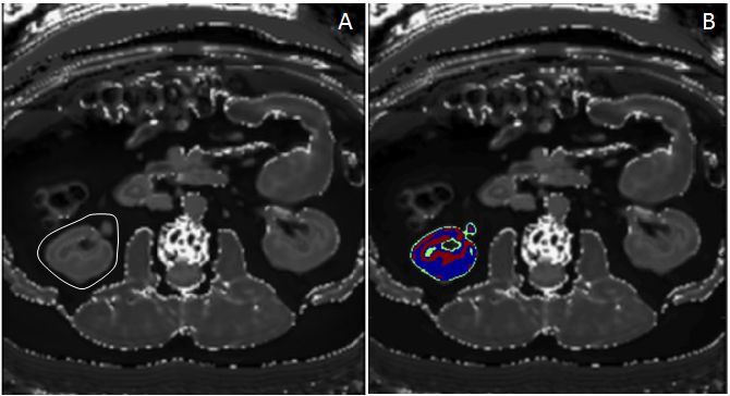
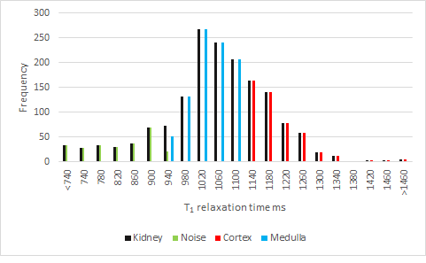
Figure 2: Shows the whole kidney ROI histogram in black and how this is divided up between the different segments with the cortex in red, medulla in blue and the noise voxels in green.