1726
Deep-Learning-Based Denoising of Diffusion-Weighted Prostate Images1Medical Physics, Memorial Sloan Kettering Cancer Center, New York, NY, United States, 2GE Healthcare, New York, NY, United States, 3Radiology, Memorial Sloan Kettering Cancer Center, New York, NY, United States
Synopsis
Despite its unique capabilities, diffusion-weighted imaging (DWI) in prostate is inherently limited by low signal-to-noise ratio (SNR). Currently, gains in SNR of high b-value images are achieved through increase in the number of excitations (NEX), at the cost of increase in total acquisition time. We demonstrate feasibility of improving prostate DWI image quality by leveraging denoising convolutional network. Using pairs of "noisy" NEX4 and "clean" NEX16 DWI images, reconstructed from raw data, CNN was trained to denoise prostate DWI images. Denoising of images significantly improved SNR and increased overall image quality, reviewed by two experienced genitourinary radiologists.
INTRODUCTION
Despite its unique capabilities in probing tissue at the cellular level, diffusion-weighted imaging (DWI) in prostate is inherently limited by low signal-to-noise ratio (SNR)1-2. In neuro MRI applications and low-dose computerized tomography, approaches to image denoising have been successfully explored3-7, but the problem of low SNR in prostate DWI has not been addressed. Currently, gains in SNR of high b-value images are achieved through increase in the number of excitations (NEX), at the cost of increase in total acquisition time. Our objective was to improve image quality of prostate DWI by leveraging denoising convolutional network (DnCNN) approach8 and exploiting the current multi-NEX DWI acquisition.METHODS
Network: In DnCNN8 (Fig. 1), noisy observation was defined as y = x + v, where x is a “clean” image, and v is noise. The goal was to train residual mapping R(y) ≈ v, so that denoised image is found as x = y – R(y). Loss function was averaged mean squared error between the “clean” and estimated denoised input images. Network depth was increased to 21, and patch size was increased to 60 × 60.
Data: Field-of-view Optimized and Constrained Undistorted Single shot (FOCUS)9 DWI is used in the standard prostate MRI protocol at our institution. Raw FOCUS data (N = 53: training-43, evaluation-5, testing-5) were retrospectively collected from six 3 T MRI scanners (GE Healthcare, Waukesha, WI) with IRB approval. Images were acquired with 3 diffusion directions, with b-valueS of 0 and 1000 s/mm2. For each direction, NEX for low b-value was 2 - 4, and for high b-value – 12 - 16.
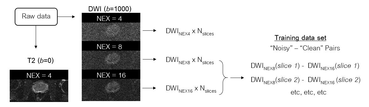
Data pre-processing (Fig 2): 1) For high b-value images, raw data were reconstructed to generate DWI images for NEX of 4, 8 and 16; low b-value images were reconstructed using all NEX and were only used for apparent diffusion coefficient (ADC) map generation. 2) For training, pairs of “noisy", DWI NEX8, and "clean”, DWI NEX16, 116 × 246 images were created. All slices were used.
Training: Using 1262 image pairs (43 patients from 5 scanners), 367,360 patches were generated. "Noisy" and "clean" images had average apparent SNR of 16.5 and 20.7. Number of epochs was 40, with 2870 iterations. The Amazon Cloud with NVIDIA K80 GPU was used.
Analysis: Trained model was applied to 5 test sets to generate denoised images for NEX of 4,8 and 16. Using unprocessed and denoised DWI images, ADC maps were computed. Apparent SNR was measured in all images. In ADC maps, the number of pixels with ADC < 0 s/mm2 was recorded. Negative ADC ratio was computed by normalizing all pixel counts by the number of negative ADC pixels in unprocessed NEX16 image, original DWI image. Two-tail paired t-test was used to compare quantitative metrics between unprocessed and denoised images. Additionally, two experienced genitourinary radiologists independently reviewed 25 randomly-paired-up unprocessed and denoised image sets. Each recorded if one set of images had better overall diagnostic quality compared to the other or if there was no perceivable difference.
RESULTS
Figure 3 shows RMSE distribution and loss function. Figure 4 shows the denoised and corresponding unprocessed DWI images. In the five test data sets, individually and on average apparent SNR was higher in denoised images for NEX4 (21.4±5.5 vs 13.1±3), NEX8 (26.7±7.6 vs 16.5±4.6) and NEX16 (25.7±7.9 vs 20.3±6.1), p < 0.001 (Fig 5A). Compared to using unprocessed NEX4 or NEX8 images to compute the ADC maps, the number of pixels with ADC < 0 s/mm2 was significantly smaller when using denoised NEX4 (p=0.02) or denoised NEX8 (p=0.002) images (Fig 5B). For 20 out of 25 reviewed image set pairs, there was agreement between the radiologists (Figure 5C): unprocessed NEX16 was preferred over unprocessed NEX8 and all denoised images were preferred over corresponding unprocessed images. In remaining 5 out of 25 reviewed pairs, comparing denoised NEX8 and unprocessed NEX16 images, radiologist 1 indicated no preference, and radiologists 2 preferred the denoised NEX8 image.CONCLUSION
Unlike brain or liver applications, where denoising has been explored and where majority of the image contains some anatomical information, the prostate DWI images consist mostly of the pixels appearing as noise (corresponding muscle or bone marrow tissue). Small fraction of the image is occupied with the structures of interest (prostate, lymph nodes, bladder etc.) Here, we showed that even these types of images can benefit from deep-learning denoising algorithms: DWI SNR, ADC map quality and overall image quality were improved. Continued development of DnCNN algorithms may further improve denoising of prostate DWI, thus potentially enabling 1) higher image quality with fewer NEX, saving scan time, 2) denoising of DWI images acquired at 1.5 T, and 3) improving accuracy of ADC map computation.Acknowledgements
We thank Francisco Godoy, M.S., for valuable discussion of the network optimization, python and tensorflow.References
1. Ning, P.; Shi, D.; Sonn, G. A.; Vasanawala, S. S.; Loening, A. M.; Ghanouni, P.; Obara, P.; Shin, L. K.; Fan, R. E.; Hargreaves, B. A., The impact of computed high b-value images on the diagnostic accuracy of DWI for prostate cancer: A receiver operating characteristics analysis. Scientific reports 2018, 8 (1), 3409. 2. Stocker, D.; Manoliu, A.; Becker, A. S.; Barth, B. K.; Nanz, D.; Klarhöfer, M.; Donati, O. F., Image Quality and Geometric Distortion of Modern Diffusion-Weighted Imaging Sequences in Magnetic Resonance Imaging of the Prostate. Investigative radiology 2018, 53 (4), 200-206.
3. Veraart, J.; Novikov, D. S.; Christiaens, D.; Ades-Aron, B.; Sijbers, J.; Fieremans, E., Denoising of diffusion MRI using random matrix theory. NeuroImage 2016, 142, 394-406.
4. You, C.; Yang, Q.; Gjesteby, L.; Li, G.; Ju, S.; Zhang, Z.; Zhao, Z.; Zhang, Y.; Cong, W.; Wang, G., Structurally-Sensitive Multi-Scale Deep Neural Network for Low-Dose CT Denoising. IEEE Access 2018, 6, 41839-41855.
5. Kadimesetty, V. S.; Gutta, S.; Ganapathy, S.; Yalavarthy, P. K., Convolutional Neural Network based Robust Denoising of Low-Dose Computed Tomography Perfusion Maps. IEEE Transactions on Radiation and Plasma Medical Sciences 2018.
6. Xie, D.; Bai, L.; Wang, Z., Denoising Arterial Spin Labeling Cerebral Blood Flow Images Using Deep Learning. arXiv preprint arXiv:1801.09672 2018.
7. Gong, E.; Pauly, J. M.; Wintermark, M.; Zaharchuk, G., Deep learning enables reduced gadolinium dose for contrast‐enhanced brain MRI. Journal of Magnetic Resonance Imaging 2018.
8. Zhang, K.; Zuo, W.; Chen, Y.; Meng, D.; Zhang, L., Beyond a gaussian denoiser: Residual learning of deep cnn for image denoising. IEEE Transactions on Image Processing 2017, 26 (7), 3142-3155. 9. 9. Saritas, E. U.; Cunningham, C. H.; Lee, J. H.; Han, E. T.; Nishimura, D. G., DWI of the spinal cord with reduced FOV single‐shot EPI. Magnetic Resonance in Medicine: An Official Journal of the International Society for Magnetic Resonance in Medicine 2008, 60 (2), 468-473.
Figures