1631

Classification of prostate cancer by radiomics

Jing Zhang¹, Yu-dong Zhang², Yang Song¹, Xu Yan³, and Guang Yang¹

¹East China normal university, Shanghai, China, ²Jiangsu Province Hospital, Jiangsu, China, ³MR Scientific Marketing, Siemens Healthcare, shanghai, China

Synopsis

Timely diagnosis and treatment could effectively reduce patient risk for clinical significant prostate cancer (PCa). In this abstract, we extracted 327 quantitative features from prostate mp-MRI images, then we used a homemade open-source tool named Feature Explorer to study combinations of radiomics algorithms and hyper-parameters in order to find the best model for classification of PCa into non-clinical–significant and clinical significant. We obtained a candidate model with AUC of 0.823, accuracy of 0.827. Four features selected for classification are easily understandable in the sense of image characteristics. Feature Explorer was demonstrated to be an efficient tool for radiomics studies.

INTRODUCTION:

Prostate cancer (PCa) is one of the most common cancer in the world and the number of patients increased significantly in recent years.^1,2,3Most of PCa with Gleason score less than 7 may remain low-risk for decades, but some PCa may deteriorate to clinical significant (CS) PCa with high fatality rate.⁴Multi-parametric magnetic resonance imaging (mp-MRI) is widely used to diagnose PCa.⁵However, experienced radiologists are often required in PCa screening with mp-MRI. In this abstract, we extracted 327 quantitative features from the prostate mp-MRI images and correlated them to PCa classfications.⁶

METHODS:

Dataset: PROSTATEx (https://doi.org/10.7937/K9TCIA.2017.MURS5CL) dataset was used in this study. It included 185 cases with T2W(TSE，0.5×0.5×3.6mm³)， DWI(SSEP，2×2×3.6mm³，b is 800s/mm²), and ADC map sequences from Siemens 3T MR scanners. Total 251 lesions (CS/NCS=68/183) were used in this study. DWI and ADC map were aligned to T2W images. A radiologist drew the region of interest (ROI) manually. We split the dataset into independent training (CS/NCS = 48/128) and testing dataset (CS/NCS = 20/55).

Radiomics Feature Extraction: We extracted 109 features from each ROI in each sequence with pyradiomics (http://pyradiomics.readthedocs.io/en/latest/index.html). Classes of the features used included Shape (19), First Order (16), Gray Level Co-occurrence Matrix (GLCM, 23), Gray Level Size Zone Matrix (GLSZM, 16), Gray Level Run Length Matrix (GLRLM, 16), Neighboring Gray Tone Difference Matrix (NGTDM, 5), Gray Level Dependence Matrix (GLDM, 14).

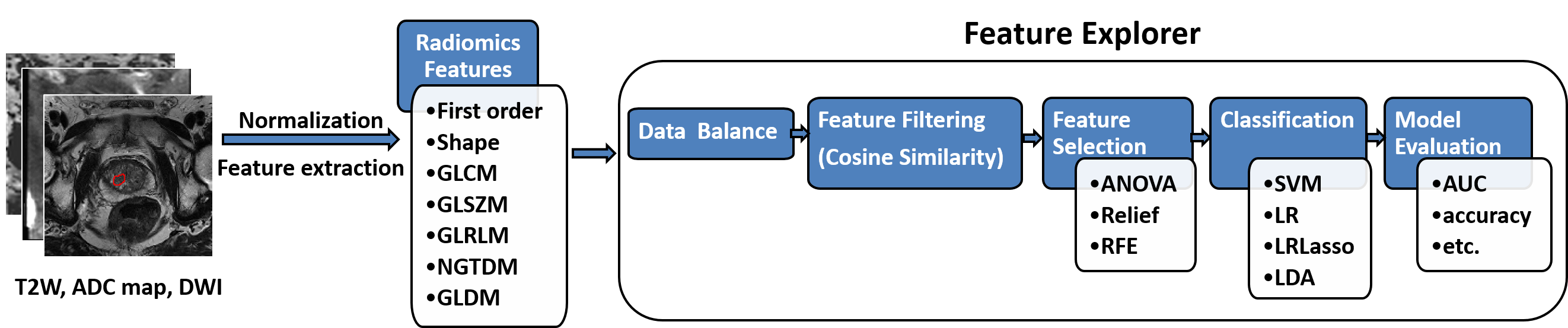
Feature Explore Pipeline: Since there are numerous number of combinations of algorithms and hyper-parameters to try out to find the best model for classification, we used a homemade open-source tool named Feature Explorer (FAE, https://github.com/salan668/FAE) to automate the process. We normalized each features, and used upsampling for data balance. Then we tried out all the combinations of three feature selection methods (ANOVA, Relief, and Recursive feature elimination) and four classifiers (SVM, LDA, Logistic Regression, and Logistic Regression with Lasso). Number of selected features was also iterated from 1 to 20. The best model was found by comparing the results of leave-one-out cross validation on the training dataset. Finally, we used receiver operating characteristic curve (ROC), area under ROC (AUC), paired t-test on the testing dataset to quantitatively evaluate the performance of the best model.

RESULTS:

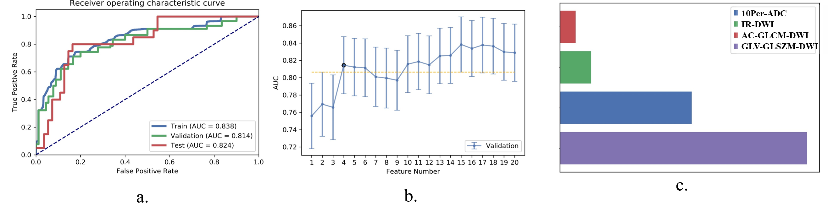
We found that the combination of ANOVA and LDA with 4 features selected yielded the best results, with AUC of 0.823, accuracy of 0.827, sensitivity of 0.800, specificity of 0.836, positive predictive value of 0.640, negative predictive value of 0.920. We showed the ROC curve of the model on training/validation/testing dataset in Figure 2 (a). The plot of the AUC on validation dataset against the number of features was shown in Figure 2 (b). 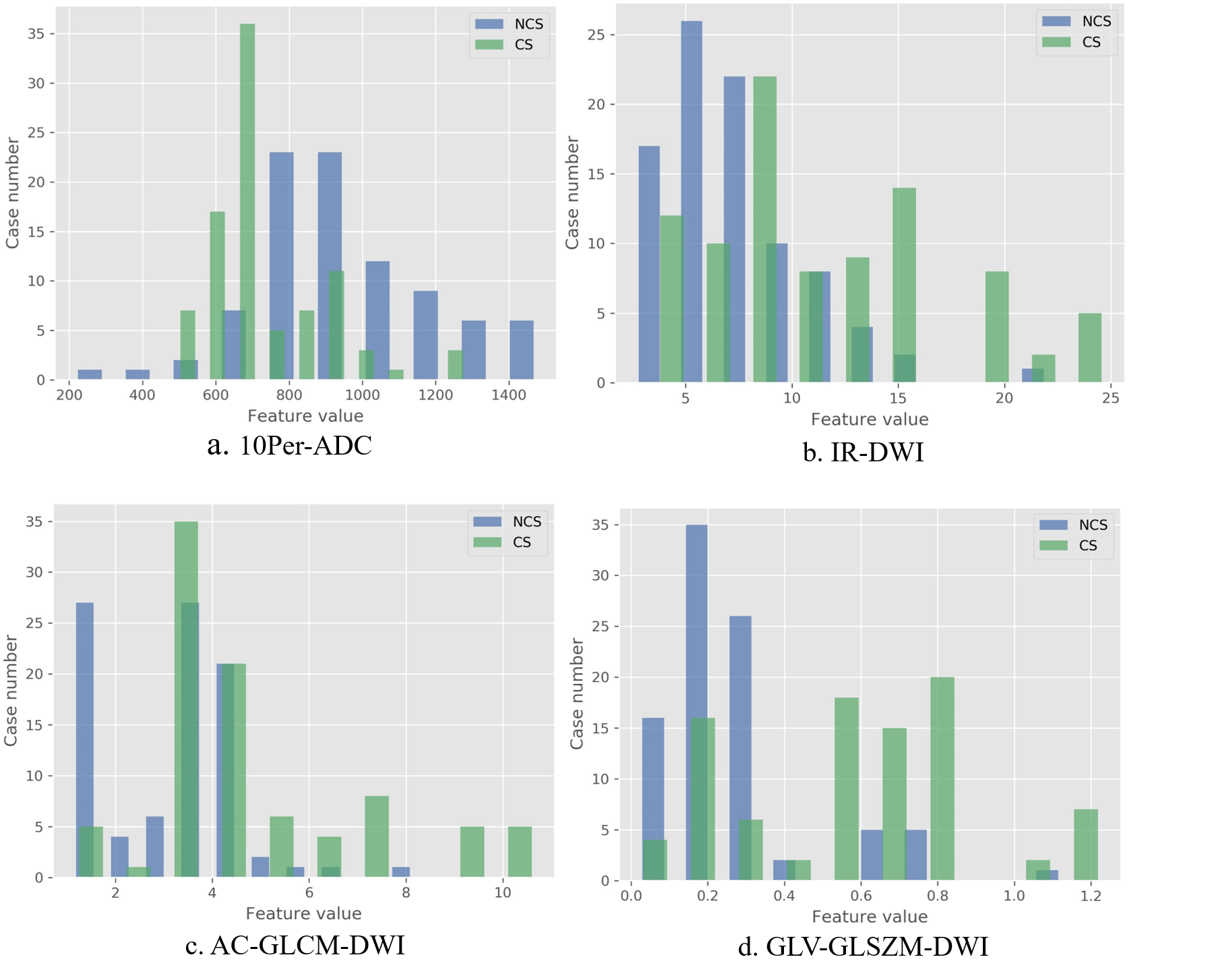The candidate number of features was determined with one-standard-error rule. The selected features were: (1) 10th percentile of ADC map (10Per-ADC), (2) the interquartile range of intensity analysis of DWI (IR-DWI), (3) auto-correlation of GLCM of DWI (AC-GLCM-DWI), and (4) the gray level variance of GLSZM of DWI (GLV-GLSZM-DWI). The contributions of these four features in the final model were shown in Figure 2. We also showed the distribution of these features of both CS and NCS PCa in Figure 3. 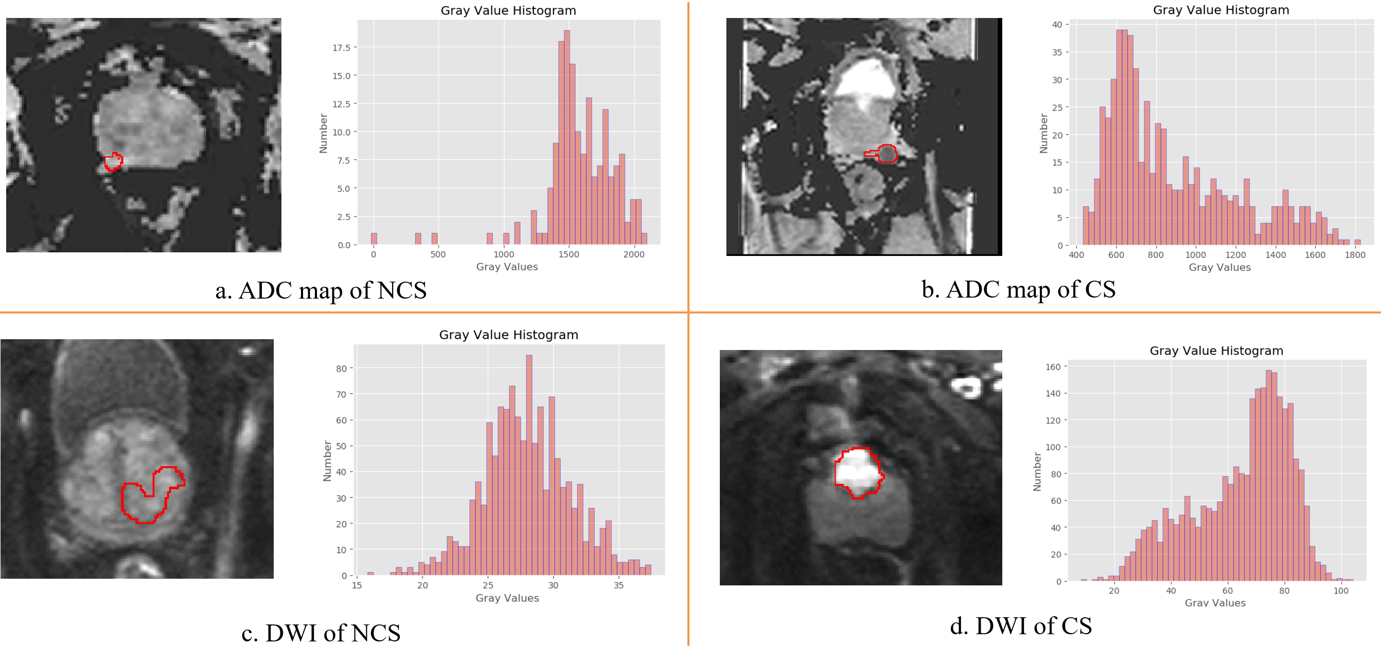The p-value of these features was smaller than 0.001 to distinguish the CS and NCS PCa. The histogram within ROI of CS and NCS PCa cases were shown in Figure 4. The features related to the histogram could be used to separate the CS and NCS PCa.

DISCUSSION:

The intensity of PCa is higher in DWI image and lower in ADC. However, to separate CS from NCS, more complex features need to be used. From the radiomics analysis, we found 10Per-ADC and IR-DWI could be used to separate CS and NCS PCa. From Figure 4 (a) and (b), we can see that the skewness of NCS and CS are negative and positive respectively. AC-GLCM-DWI, which reflected fineness and coarseness of texture, had higher values in DWI of CS PCa, indicating CS PCa tends to have coarser texture. GLV-GLSZM-DWI is also higher in CS, which means CS PCa is more inhomogeneous in gray level intensities. Though none of the above features can separate CS from NCS, the model combining all these 4 features could help to diagnose the CS PCa.

CONCLUSION:

With the help of a homemade radiomics software, Feature Explorer, we found the best model for PCa classification. Four features, each associated with certain image characteristics and easily understandable, were found to be most relevant to CS/NCS classification.

Acknowledgements

This project is supported by National Natural Science Foundation of China (81771816,61731009).

References

1.Canadian Cancer Society, Prostate Cancer Statistics, 2015.

2.American Cancer Society, Cancer Facts & Figures 2015.

3.A. Jemal, F. Bray, M. M. Center, J. Ferlay, E. Ward, and D. Forman, CA: a cancer journal for clinicians: Global cancer statistics, 2011; vol. 61, no. 2, pp. 69–90.

4.A. Stangelberger, M. Waldert, and B. Djavan, Prostate cancer in elderly men, Rev. Urol, 2008; vol. 10, no. 2, pp. 111–119.

5.Y. Peng et al. Quantitative analysis of multiparametric prostate MR images: Differentiation between prostate cancer and normal tissue and correlation with Gleason score—A computer-aided diagnosis development study, Radiology, 2013; vol. 267, no. 3, pp. 787–796.

6.P. Lambin, E. Rios-Velazquez, R. Leijenaar, S. Carvalho, et al. Radiomics: extracting more information from medical images using advanced feature analysis, European Journal of Cancer, 2012; vol. 48, no. 4, pp. 441–446.

Figures

Figure 1 : Radiomics analysis flowchart. We normalized gray level in all images before feature extraction. Features were extracted with pyradiomics. All those extracted features will be filtered with cosine-similarity before feature selection algorithms were used to select relevant features. Survived features were then used to train the classifier. All the processing after feature extraction were performed in FeatureExplorer.

Figure 2: The optimal model found by FAE, in which ANOVA is used for feature selection, and LDA as classifier. Four features were selected by the model. (a) ROC curve of the optimal model with Train AUC of 0.838, Validation AUC of 0.814, Test AUC of 0.824. (b) The plot of the AUC value against the number of features. We used one-standard-error rule to find the candidate number of features. (c) Contributions of the selected features, namely 10Per-ADC (weight value in LDA is -7.98), IR-DWI (weight value in LDA is 1.89), AC-GLCM-DWI (weight value in LDA is 0.95), GLV-GLSZM-DWI (weight value in LDA is 14.96).

Figure 3.The histograms of the 4 most important features: The blue and green bars denote NCS and CS PCa, respectively. It can be seen that 10Per-ADC tends to have lower values in CS while IR-DWI, AC-GLCM-DWI, and GLV-GLSZM-DWI tend to have higher values in CS. The p-values of all 4 features to distinguish CS/NCS are less than 0.001.

Figure 4. CS/NCS images and corresponding histograms of ROI. As seen in ADC maps in (a) (b), cancer region features higher signal in NCS and histograms of NCS and CS show opposite skewness. As seen from DWI images in (c) (d), cancer region in NCS has lower intensities and narrower distribution in histogram.

Proc. Intl. Soc. Mag. Reson. Med. 27 (2019)

1631