Synopsis

Here we present an improved method for ZTE to pseudo CT conversion by combining an analytical signal model (i.e. ZTE to CT signal scaling) with Connected Component Analysis (CCA) and Deep Learning (DL) based air vs. bone discrimination. The method is demonstrated for the two main anatomical regions (head&neck and pelvis) and the two main field strengths (1.5T and 3T) of interest.

Introduction

Converting MR images into X-ray attenuation information is an important prerequisite for emerging applications including MR-guided Radiation Therapy Planning (MRgRTP) and PET/MR attenuation correction (PET/MR-AC). While MRI shines in depicting soft-tissues (including fat-water separation using Dixon type methods), capturing MR bone signal and differentiating it against air remains challenging.

Recently we demonstrated proton density (PD) weighted Zero TE (ZTE) for bone imaging and pseudo Computed Tomography (CT) image conversion in the head (1,2). Here we present an improved method for ZTE to pseudo CT conversion by combining an analytical signal model (i.e. ZTE to CT signal scaling) with Connected Component Analysis (CCA) and Deep Learning (DL) based air vs. bone discrimination. The method is demonstrated for the two main anatomical regions (head & neck and pelvis) and the two main clinical field strengths (1.5T and 3T) of interest.

Methods

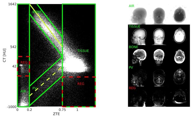
The left side of Fig. 1 illustrates a 2D histogram of registered CT vs. ZTE signals and its right side shows anatomical regions corresponding to clusters in the histogram (i.e. air, tissue, bone and partial volume (PV)). Air (CT≈-1000HU) and soft-tissue (CT≈+50HU) are well separated and can be robustly identified by ZTE<0.2 and ZTE>0.75, respectively. As can be seen from the histogram, ZTE bone and PV signals scale linearly to CT Hounsfield units (2):

$$CT_{BONE}=-2000*(ZTE_{BONE}-1)+42, \space and \space CT_{PV}=min(1042/0.75*ZTE_{PV}-1000,42) \space [1]$$

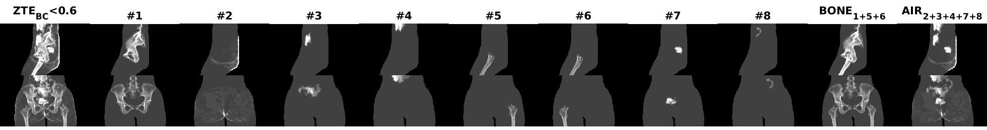
Bone and PV regions are overlapping (0.2<ZTE<0.75) and cannot be distinguished based on signal intensity alone. Instead bone and PV are separated using structural neighborhood information. For the pelvis region (where bone and PV regions are not in direct contact) a Connected Component Analysis (CCA) was performed to identify major bones (pelvic bone, femur, spine) and distinguish them from abdominal PV regions (cf. Figure 2).

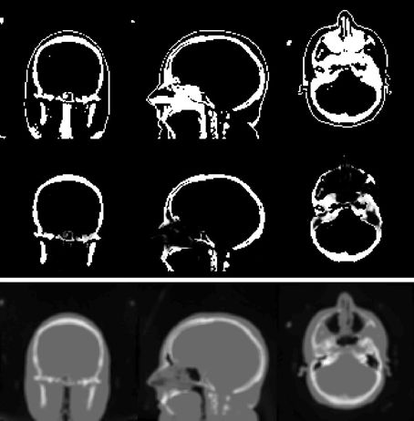
In the head & neck region (including complicated bone-tissue-air interfaces like the sinus cavities) a fully connected neural network was used. More specifically, for each ambiguous voxel (0.2<ZTE<0.75), ZTE signals of an encapsulating 3D spherical patch (diameter=60mm) are interpolated to 2.4mm, flattened and feed into a 6-layer, fully-connected neural network (i.e. 8126_INPUTx128_HIDDENx128_HIDDENx128_HIDDENx128_HIDDENx1_OUTPUT nodes using rectified linear units (ReLu) and a sigmoid activation function at the end). The Deep Learning was trained based on N=157 ZTE and corresponding pseudo CTs obtained from a previously described method (3) including manual refinements.

MR imaging was performed on 1.5T MR450w and 3T MR750w scanners using GEM surface coils (GE Healthcare, Chicago, IL). ZTE imaging parameters were chosen identical for head&neck and pelvis (i.e. FOV=(500mm)³, res=(2mm)³, FA=1°, BW=±62.5kHz, NEX=4, scan time ~5mins). For the pelvis an additional 3D GRE Dixon-type LAVA-Flex sequence was acquired for fat-water separation. All image processing was implemented in Matlab (MathWorks, Natick, MA), and tested for ZTE to pseudo CT conversion in the head&neck and pelvis at 1.5T and 3T. The processing time for 3D ZTE to pseudo CT image conversion (including DICOM reading) was ~30s.

Results and Discussion

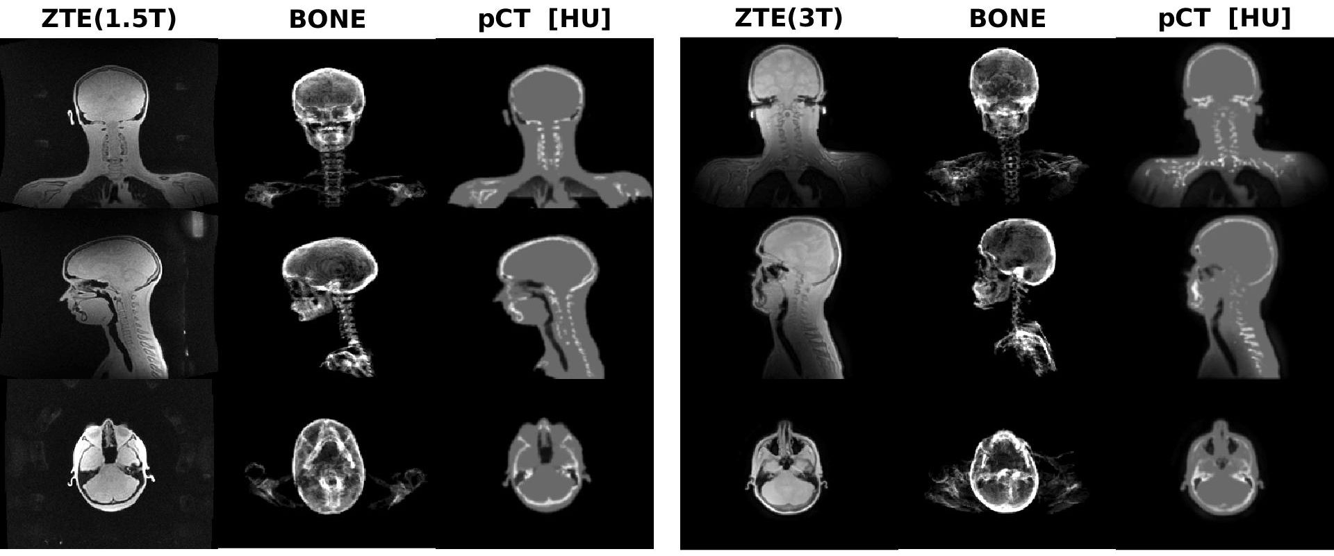
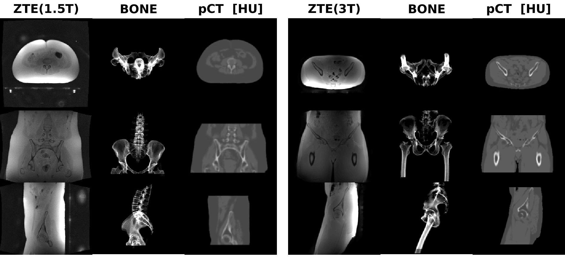
Figure 4 shows head & neck results for 1.5T (left subplot) and 3T (right subplot), including the original input ZTE image (left), the MIP bone mask (middle) and the obtained pseudo CT in Hounsfield units (right). The obtained results indicate clean bone depiction in the head and neck area. The shoulder and lung region indicates some bone misclassification due to lower SNR and that anatomy not being present in the training.

Figure 5 illustrates pelvic results using the same formatting as in the previous figure. All major bones (i.e. pelvic bone, femur, spine) are well captured. The LAVA-Flex images provide additional fat-water discrimination.

Generally, 1.5T ZTE images appear sharper compared to corresponding 3T ones. This is a consequence of the fat-water chemical shift off-resonance which linearly increases with field strength causing undesired blurring and signal interferences at 3T (4).

The presented ZTE to pseudo CT image conversion method combines analytical signal conversion (cf. Eq. [1]) with CCA and Deep Learning to resolve low ZTE signal regions into bone and PV regions. Different to earlier DL-based MR to CT image conversion approaches, the described method is two orders of magnitude faster by just focusing on the bone-air ambiguity (~30s processing time), thereby obviating the need for dedicated GPUs. Finally, the presented method can be trained using MR data only.

Acknowledgements

References

1) Wiesinger et al, Zero TE MR bone imaging in the head. MRM 75: 107-114 (2016).

2) Wiesinger et al, Zero TE-based pseudo-CT image conversion in the head and its application in PET/MR-AC and MR-guided RTP. MRM 80: 1440-1451 (2018).

3) Kaushik et al, Deep Learning based pseudo-CT computation and its application for PET/MR-AC and MR-guided RTP, ISMRM Paris: p.1253 (2018).

4) Engström et al, Perfect In-Phase Zero TE for Musculoskeletal Imaging, ISMRM 2019: submitted.