1524
Full Wave vs Quasistatic Simulation Accuracy at 3 Tesla1Radiology, University of Utah, Utah Center For Advanced Imaging Research (UCAIR), SALT LAKE CITY, UT, United States
Synopsis
Full wave simulations are known for their high accuracy, but simulation optimization is not feasible with FDTD and FEM for vast numbers of MRI coil applications. Optimization strategies do have feasible runtimes for quasi-static solutions, but the system being simulated must be small compared to the electromagnetic wavelength since they do not account for boundary conditions. This work uses multiple single loop coils of different diameters and three phantoms with a simple geometry to compare the accuracy and usefulness of full wave and quasi-static solutions of RF coils at 3T. Full wave simulations proved to be significantly more accurate.
Purpose:
Though computing power has significantly increased, the runtime of full wave simulations—such as the finite difference time domain (FDTD) and finite element method (FEM)—can make optimization algorithms utilizing them impractical. Quasi-static simulations offer practical run times, but they assume that the system being simulated is small compared to the electromagnetic wavelength for accurate solutions1. Full wave solutions do not have this limitation since they exploit the full Maxwell equations which include boundary conditions and radiative losses. This work uses multiple single loop coils of different diameters, and three phantoms with a simple geometry and varying conductivity, to compare the accuracy and usefulness of full wave and quasi-static solutions for RF coils at 3T. Benchtop measurements and imaging experiments are used as gold standards.Methods:
Three cylindrically shaped phantoms, Fig 1, were used with solutions of 1.955g CuSO4 x H20 combined with 1.094g NaCl, 3.020g NaCl, and 4.915g NaCl to achieve 0.3, 0.6, and 0.9S/m conductivities (at 20°Celsius), respectively. The phantom height and radius were 10.1 and 13.9cm.
Eight circular 16 AWG copper wire coil loops ranging from 3-10cm in diameter in 1cm increments were constructed for each phantom (24 total). The coils had 1, 2, 3, and 4 tune capacitors for the 3,4cm, 5,6cm, 7,8cm, and 9,10cm diameter loops, respectively. Coils were tuned and matched to the same impedance. The preamplifier socket connected directly to the match circuit, eliminating a cable. The same preamplifier was used for all measurements.
SNR measurements were acquired using 2D axial GRE sequences positioned through the center of each coil with noise calculated as the standard deviation of noise-only image voxels. Images were acquired on a 3T MRI scanner (MAGNETOM Tim Trio, Siemens Healthcare, Erlangen, DE).
Full wave simulations were performed using Computer Simulation Technology Microwave Studio (CST MWS). The FDTD method was used with mesh cell counts ranging from 2-11 million mesh cells, simulation accuracy of -80dB, and an “Enhanced (Preview)” AR-filter with a max error for steady state of 0.001. CST Design Studio (DS) co-simulation was used to tune the coils and calculate the composite magnetic field (B1-) and total noise (Rt)2-4. Total noise was calculated by removing the match capacitor and measuring the real part of the Z1,1 parameter. The active decoupling diode on the match circuit between the signal and ground was included in the CST simulations as a 0.8pF capacitor. Total MWS run times ranged from 24m to 4h22m per coil.
Quasi-static simulations used Biot-Savart for magnetic field calculations and vector potential for noise calculations5. Calculations of sample resistance (Rs) and coil resistance (Rc) were done separately and total noise was calculated by Rt = Rs+Rc. Run time was less than 4 seconds per coil.
Total noise bench measurements were made using the same method used for the full wave measurements3.
Preamplifier noise was not included in any of the noise calculations or measurements. Full wave and quasi-static SNR results were scaled (one scaler for each method) to make the SNR calculations of the 3 cm loop on the 0.3S/m phantom match that of the SNR measurement at 8 cm depth from the loop center. We assumed a uniform body coil excitation.
Results:
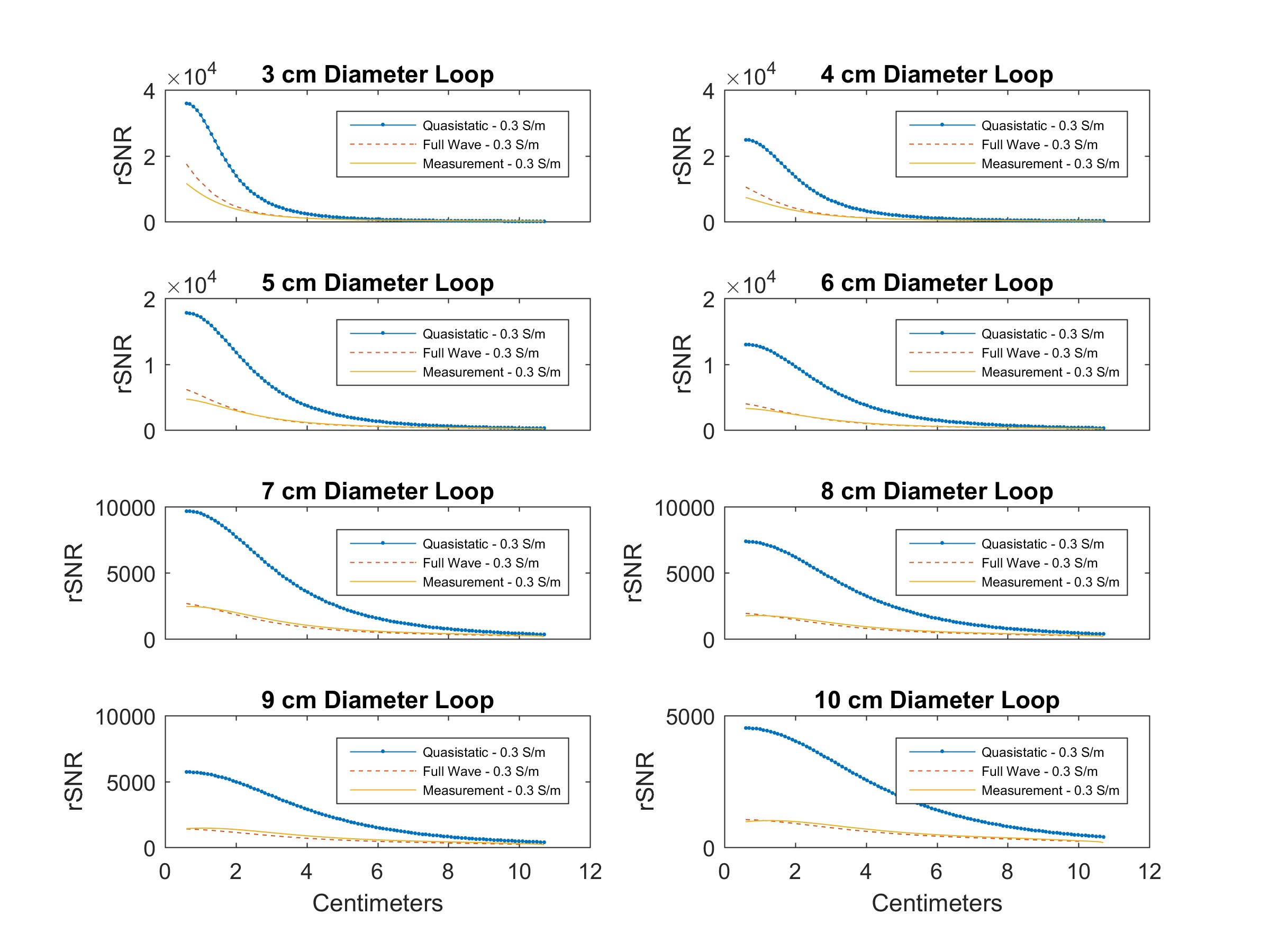
SNR plots for the 6cm loops are shown in Fig 2. SNR line plots through the axis of the coil are shown in Fig 3-5. Noise measurements are shown in Fig 1. The full wave and quasi-static total noise calculations ranged from 1.06-0.83 and 3.02-0.27 from the bench measurements, respectively.Discussion:
The full wave simulations correctly represented the signal and noise while the quasi-static simulations did not. Superficial B1- discrepancies in the full wave simulation were mainly due to flip angles not being 90° in the phantom. Discrepancies in the quasi-static signal and noise are largely due to the assumption that boundary conditions are correctly accounted for at infinity1. The quasi-static method did not accurately calculate B1- nor did it account for the increase in noise with coil diameter for the 0.3S/m phantom. This anomalous increase was due to a larger electric field strength for coils larger than 7 cm when compared to that in the 0.6 and 0.9S/m phantoms.
We have demonstrated that the frequency at 3T is high enough for a large system to have destructive wave effects, requiring a full wave simulation for accurate results. Further work would include whether a system that is small compared to the electromagnetic wave could be accurately characterized with a quasi-static solution or if a software package like MARIE using integral equations is necessary and/or practical for all optimizations at 3T6.
Acknowledgements
No acknowledgement found.References
1. Larsson, Jonas. Electromagnetics from a quasistatic perspective. Am. J. Phys. 2007;75(3):230-239.
2. Hoult, D.I. The principle of reciprocity in signal strength calculation-A mathematical guide. Concepts Magn Reson. 2000;12(4):173-187.
3. Lemdiasov et al. A numerical post processing procedure for analyzing radio frequency MRI coils. Concepts Magn Reson Part A. 2011;38A(4):133-147.
4. Horneff et al. An EM simulation based design flow for custom-build MR coils incorporating signal and noise. IEEE Trans Med Imaging. 2018;37(2):527-535.
5. Roemer et al. The NMR phased array. Magn Reson Med. 1990;16(2):192-225.
6. Villena et al. Fast Electromagnetic Analysis of MRI Transmit RF Coils Based on Accelerated Integral Equation Methods. IEEE Trans Biomed Eng. 2016;63(11):2250-2261.
Figures

Fig 1: Top, cylindrical shaped phantom, 10.1 (height) and 13.9cm (radius), used for experiments. There were three total phantoms with 0.3, 0.6, and 0.9S/m. Bottom, total noise (Rt) for the quasi-static, full wave, and measurements. The full wave and measurement noise values included an active decoupling diode on the match circuit, between the signal and ground, which increases the total noise by approximately 15-30% compared to the match circuit without the diode.