Synopsis

A simple and easy to implement method for shim coil design is proposed as an alternative to most popular, but complicated methods. It is straightforward in obtaining the optimal stream function, which is further discretized into a coil wiring, using an analogy to magnetized material and a boundary discretization into square dipoles. Simulation results show good performance in designing spherical harmonics shim coils.

Introduction

Magnetic field shimming is usually performed by independent shim coils that create spherical harmonic fields inside the DSV.

Shim coils are generally designed by methods such as the Target Field Method¹ or the Inverse Boundary Element Method². However, TFM needs solving laborious Fourier-Bessel integrals while IBEM is based on a triangular mesh discretization that might not be necessary if designing shim coils over a cylindrical or biplane coil former.

To design a coil that will generate a target magnetic field $$$B_z(\mathbf{x})$$$ inside a region $$$\mathcal{V}$$$, either a surface current density $$$\mathbf{j}(\mathbf{x})$$$ or its stream function³ over a conductive coil former $$$\mathcal{S}_c$$$ needs to be calculated. The stream function is usually more convenient, since it can easily be used for discretization into wires for coil design³.

We propose a simple method for shim coil design derived from an analogy with magnetized materials generating the target field. It provides a straightforward stream function defining the wire paths to generate the target field.

Theory and methods

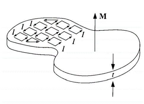
A magnetized material possesses a magnetization $$$\mathbf{M}$$$ within its volume, which generates a magnetic field in space. The magnetized region can be considered as a distribution of many dipoles as shown in Figure 1.

Let $$$d\mathbf{m}(\mathbf{x})$$$ be the magnetic dipole moment in a volume cell $$$dV$$$ of thickness $$$t$$$ and area $$$dA$$$, located at $$$x$$$ on $$$\mathcal{S}_c$$$, and $$$I(\mathbf{x})$$$ be the dipole current around $$$dA$$$. Then:

$$\mathbf{M}(\mathbf{x})=\frac{d\mathbf{m}(\mathbf{x})}{dV}=\frac{I(\mathbf{x})dA}{tdA}=\frac{I(\mathbf{x})\mathbf{\hat{n}}(\mathbf{x})}{t}$$

The volume current density $$$\mathbf{J_b}(\mathbf{x})$$$ called bound current, which represents the capacity of the magnetization of generating magnetic field in space, is calculate by:

$$\mathbf{J_b}(\mathbf{x})=\nabla\times\mathbf{M}(\mathbf{x})$$

Moreover, $$$\mathbf{J_b}$$$ is simply related to $$$\mathbf{j}$$$ by: $$$\mathbf{j}(\mathbf{x})=\mathbf{J_b}(\mathbf{x})t$$$

By combining the three above equations, $$$\mathbf{j}(\mathbf{x})$$$ becomes:

$$\mathbf{j}(\mathbf{x})=\nabla{}I(\mathbf{x})\times\hat{\mathbf{n}}(\mathbf{x})$$

From this equation and the definition of the stream function³, it follows that $$$I(\mathbf{x})$$$ is a stream function for $$$\mathbf{j}(\mathbf{x})$$$ over the surface $$$\mathcal{S}_c$$$.

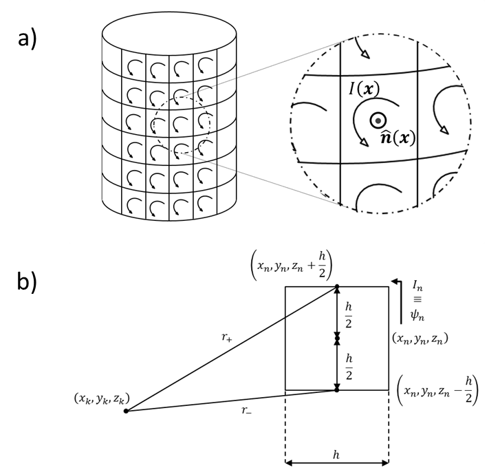
Now let us specify $$$\mathcal{S}_c$$$ as a cylinder of length $$$L$$$ and radius $$$a$$$. It can be discretized into a mesh of $$$N$$$ small square current loops of side $$$h$$$, thus obtaining a boundary composed of magnetic dipoles (Figure 2a).

The magnetic field in a point $$$\mathbf{x}_k$$$ of $$$\mathcal{V}$$$ generated by the n^th square loop of current $$$I_n$$$ can be calculated from Biot-Savart Law, if $$$h$$$ is sufficiently small, as:

$$\tilde{b}_k^n\approx{}\left[\frac{\mu_0}{4\pi}(a^2-x_n{}x_k-y_n{}y_k)\left(\frac{1}{r_-^3}-\frac{1}{r_+^3}\right)\frac{h}{a}\right]I_n$$

with (Figure 2b)

$$r_\pm = \sqrt{(x_k-x_n)^2+(y_k-y_n)^2+\left(z_k-\left(z_n\pm\frac{h}{2}\right)\right)^2}$$

$$\tilde{b}_k^n=p_{k,n}I_n$$

Adding the contributions of each square loop of the coil former,

$$\tilde{b}_k=\sum_{n=1}^{N}p_{k,n}I_n$$

$$\tilde{\mathbf{b}}=\mathbf{P}\mathbf{I}$$

where

$$\tilde{\mathbf{b}}=[\tilde{b}_1\;{}\tilde{b}_2\;{}...\;{}\tilde{b}_k]^T$$

$$\mathbf{I}=[I_1\;{}I_2\;{}...\;{}I_N]^T$$

From Maxwell's equations the power consumption of the coil can be derived from:

$$\mathcal{P}=\int_{\mathcal{V}_c}\frac{|\mathbf{J_b}|^2}{\sigma}\,dv=\int_{\mathcal{S}_c}\frac{|\nabla{}I(\mathbf{x})\times\hat{\mathbf{n}}(\mathbf{x})|^2}{t\sigma}\,dv$$

$$\mathcal{P}\approx\frac{1}{t\sigma}\sum_{n=1}^{N}\left[(I_{n+1}-I_n)^2+(I_{n+n_{\phi}}-I_n)^2\right]$$

with $$$\sigma$$$ being the coil conductivity and $$$n_\phi$$$ the number of square loops along a cylindrical row. In matrix form:

$$\mathcal{P}\approx\mathbf{I}^T{}\mathbf{R}\mathbf{I}$$

Let $$$\mathbf{b}=[b_1\;{}b_2\;{}...\;{}b_k]^T$$$ be the target field $$$B_z(\mathbf{x})$$$ in $$$K$$$ control points. The stream function $$$\mathbf{I}$$$ that best generates this field while maintaining low power consumption is:

$$\mathbf{I}(\lambda)=\underset{\mathbf{I}\in\mathbb{R}^N}{\mathrm{argmin}}\,|\mathbf{b}-\mathbf{P}\mathbf{I}|_2^2+\lambda{}\mathbf{I}^T\mathbf{R}\mathbf{I} $$

where $$$\lambda$$$ is a regularization parameter.

Then,

$$\mathbf{I}=(\lambda{}\mathbf{R}+\mathbf{P}^T\mathbf{P})^{-1}\mathbf{P}^T\mathbf{b}$$

from which a cylindrical winding can be found.

A shim coil is typically designed to address a particular spherical harmonic function $$$[l,m]$$$ of order $$$l$$$ and degree $$$m$$$.

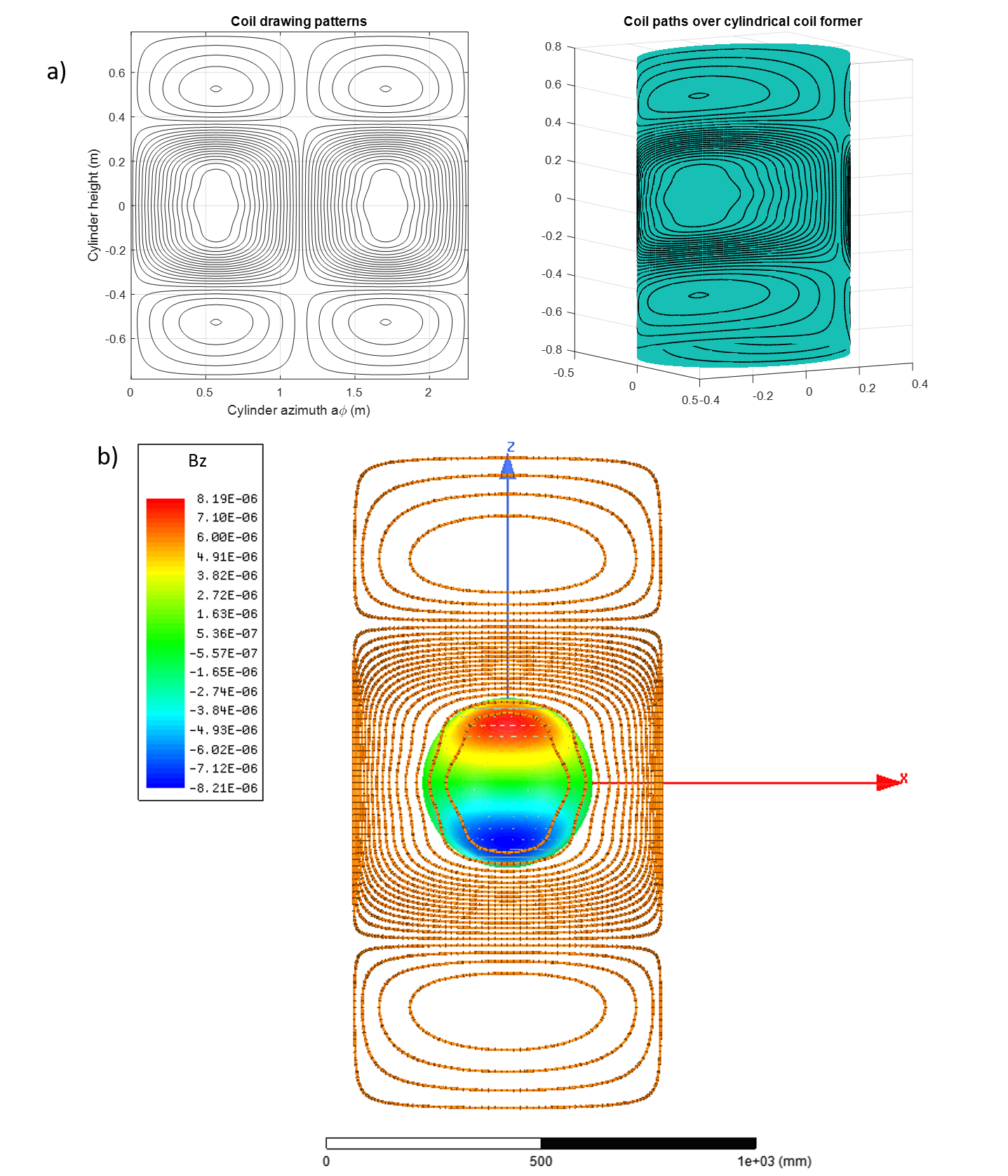
To validate our computational method on an example, design of a [2,-1] (ZY) shim coil was performed under MATLAB^®, and the resulting field computed in ANSYS^® Electronics Desktop Electromagnetism Suite.

Cylindrical coil former had 1580-mm and 362-mm radius and was discretized with square elements of 15-mm side. Nominal shim strength was chosen as 7.2mT/m² at 30A and regularization parameter was set to 10^-13. A total of 10201 control points were regularly sampled over the surface of a 40-cm DSV. Copper conductor of 8-AWG was used.

The resulting magnetic field is post-processed to confirm fidelity with the target field. To evaluate field error between $$$\mathbf{b}$$$ and $$$\mathbf{\tilde{b}}$$$, the following metric is used:

$$\varepsilon=\frac{1}{max|b_k|}\sqrt{\sum_{k=1}^{K}\frac{(b_k-\tilde{b}_k)^2}{K}}$$

Results

Coil generation in MATLAB^® provided the design showed in Figure 3a. ANSYS^® simulation model is in Figure 3b.

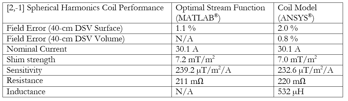
Simulation results are listed in Table 1.

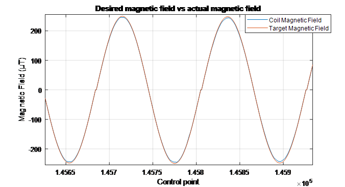
Figure 4 shows the expected vs computed magnetic field at some control points.

Discussion and conclusion

From the simulation results, the Dipole Boundary Method (DBM) performed well in designing the [2,-1] shim coil, with only 2% field error inside the DSV.

ANSYS® results showed a slightly lower sensitivity for the coil, most likely due to the wire discretization imperfections.

Lower values for coil resistance could be obtained if the regularization parameter was increased, but field error would increase, thus a compromise must be found depending on the application.

Overall, the DBM is a simple alternative for designing shim coils. Increments in the algorithm could be brought to design shielded gradient coils with minimal inductance.

Acknowledgements

References

1. R. Turner. A target field approach to optimal coil design. Journal of Physics D: Applied Physics, 1986; 19 L147

2. M. Poole, R. Bowtell. Novel gradient coils designed using a boundary element method. Concepts Magn. Reson., 31B, 2007; 162-175.

3. G.N. Peeren. Stream function approach for determining optimal surface currents. Journal of Computational Physics, 2003 Oct; 191(1):305-321