Synopsis

We explore the use of small permanent magnets moving along prescribed helical paths for spatial encoding in ultra-low field magnetic resonance systems based on Halbach arrays. A semi-analytical simulation method was developed to analyse different magnet path and orientations. For proof-of-concept, different helical magnet paths and lengths for one and two small magnets were considered to establish spatial encoding efficiency. We demonstrate that a single small encoding magnet moving around the sample in a single helical revolution can be used to generate 3D images via the method of back projection for image reconstruction.

Introduction

Methods

The ULF-MRI instrument with the encoding array: Fig.1 illustrates the design of an SPMA based ULF-MRI system. It comprises four concentrically arranged cylindrical magnet arrays: Array A with individually rotatable magnets for switching the pre-polarization field Bp which generates sample magnetization; Arrays B and C for generating the measurement field Bm; and the Encoding Array D with two permanent magnets (a-b) that creates 3D spatial encoding fields Be.

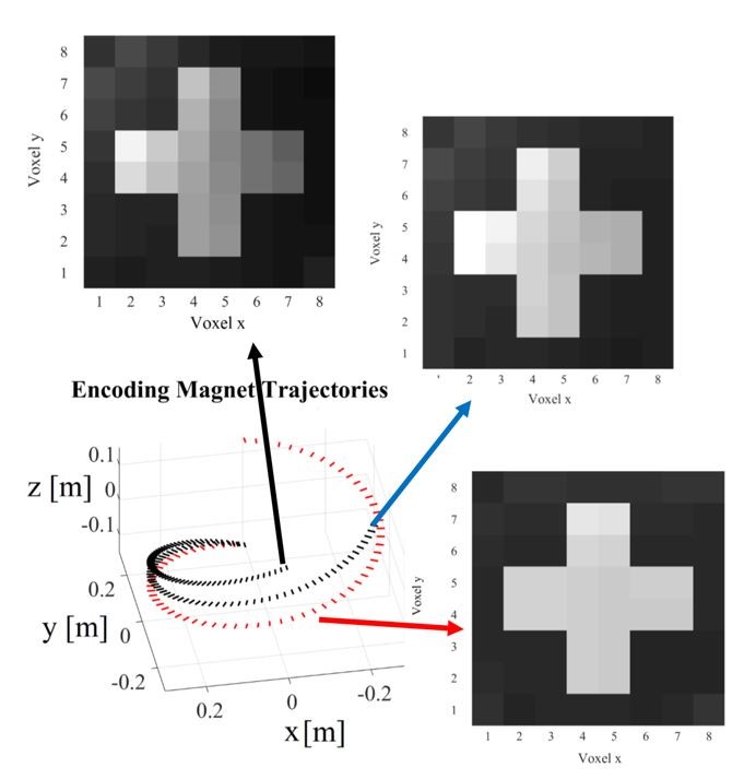
Simulation environment: COMSOL© was used to estimate the temporal field evolution from pre-polarization to measurement. Spin evolution, signal detection and image reconstruction simulations were performed in MatLab©. A 3D cubic cross-shaped digital phantom (8x8x8 voxels)(Fig.5) was employed using typical soft tissue relaxation times at ULF (T1=100ms and T2=80ms)⁴.

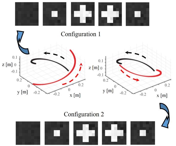
Acquisition strategy: The encoding field configurations are generated by Array D with each encoding magnet moving along a prescribed path in discrete steps. For a total of Q voxels in a sample and N time points, we used Q/N different encoding field configurations. In our simulations we used 64 encoding steps to solve the 512 voxels of the 3D phantom. We examined encoding field configurations generated by magnet paths that were feasible for the ULF-MRI instrument design. We considered the case of one and two identical magnets moving along different path configurations (Fig.2&5).

Evaluation of encoding field configuration: We aimed to maximize the rank of the encoding matrix, which reflects the number of linearly independent rows. We also aimed for a low condition number, which determines the accuracy of the numerical matrix solvers.

Results

One encoding magnet: Fig.3 shows the condition number of the encoding matrix versus the encoding magnet orientation. Three values for α₂ were selected: 180^o (Fig.3A), 100^o (Fig.3B) and 230^o (Fig.3C). Condition number significantly increased as path length decreases but varies by less than one order of magnitude for α₃ between 240^o and 360^o. Greater path length results in a lower standard deviation between reconstructed and phantom images: standard deviation = 0.0231 for α₃=180^o, 0.0221 for α₃=240^o and 0.0200 for α₃=360^o (Fig.4). Besides, a linearly descending trajectory improves performance (Fig.2).

Two encoding magnets: The optimal orientation angles for the two magnets are perpendicular to the magnet path (φ₁^opt and φ₂^opt~0^o) and parallel to the xy-plane (θ₁^opt and θ₂^opt~0^o). The reconstructed images for each configuration are shown in Fig.5. The standard deviations for configurations 1 and 2 were 0.0254 and 0.0287 respectively; image quality was higher in the former.

Discussion

Shortening the path length reduced the step size, leading to an increased linear dependence between encoding field configurations. Hence, image quality is degraded if the encoding magnet does not revolve completely around the sample. For the configurations considered, the optimal magnet orientations were perpendicular to both the motion path and the cylindrical surface of Array D. This is a consequence of the torus-shaped magnetic field distribution of a magnetic dipole⁵.

The lowest condition numbers were achieved when z(α) was a linear function of α. This is attributed to the low helical path slopes for the nonlinear height variation near the bottom (black curve, α₂=100^o) and the top (blue curve, α₂=240^o; see Fig.2) which lead to lower variation in the encoding field along the z-axis and hence increased linear dependencies and higher condition numbers.

The generated encoding field strength in the field of view ranged between 1-10µT, corresponding to a frequency spread of 43-430Hz, well within the bandwidth of coil-based magnetometers⁶.

Although only spiral paths with equidistant stopping points along a cylindrical surface were considered, the semi-analytical method can readily be extended to include any number of magnets moving along any prescribed paths.

Conclusion

Acknowledgements

References

1. Vogel, M. W., Giorni, A., Vegh, V., Pellicer-Guridi, R. & Reutens, D. C. Rotatable Small Permanent Magnet Array for Ultra-Low Field Nuclear Magnetic Resonance Instrumentation: A Concept Study. PloS one 11, e0157040 (2016).

2. Cooley, C. Z. et al. Two‐dimensional imaging in a lightweight portable MRI scanner without gradient coils. Magnetic resonance in medicine 73, 872-883 (2015).

3. Cooley, C. Z., Stockmann, J. P., Sarracanie, M., Rosen, M. S. & Wald, L. L. in Intl Soc Mag Res Med. 4192.

4. Zotev, V. S. et al. SQUID-based microtesla MRI for in vivo relaxometry of the human brain. IEEE Transactions on Applied Superconductivity 19, 823-826 (2009).

5. Cheng, D. K. Field and wave electromagnetics. (Addison-Wesley, 1989).

6. Pellicer-Guridi, R., Vogel, M. W., Reutens, D. C. & Vegh, V. Towards ultimate low frequency air-core magnetometer sensitivity. Scientific reports 7, 2269 (2017).