1450

Calibrated Coil Combination for Fixed-Geometry, Low-Frequency Coils with Application to Hyperpolarized 13C Measurements

Juan Diego Sánchez Heredia¹, Rie B. Hansen¹, Rafael Baron¹, Esben S. Szocska Hansen², Daniel H. Johansen¹, Vitaliy Zhurbenko¹, Christoffer Laustsen², Lars G. Hanson¹, and Jan H. Ardenkjær-Larsen¹

¹Department of Electrical Engineering, Technical University of Denmark (DTU), Kgs. Lyngby, Denmark, ²MR Research Centre, Department of Clinical Medicine, Aarhus University, Aarhus, Denmark

Synopsis

We explore a new design approach for low frequency RF coils, where a transmit and receive array are built together in a totally rigid frame, and therefore their B₁⁺ and B₁^- distributions can be accurately mapped and used as prior information for SNR-optimal combination of signals from different coil elements. Using this principle, a coil is designed for ¹³C MRS of a pig at 3T (32.13 MHz). We show that at this frequency, the effect of sample loading is minimal, and the prior information obtained in phantoms benefits in-vivo experiments. This one-time calibration allows for optimal combination of coil signals, which is also expected to improve parallel imaging performance.

Introduction

Flexible RF coil arrays are widely used in clinical MRI due to their superior anatomical fitting and patient comfort. However, at low frequencies, coil flexibility comes with the price of a higher thermal noise (e.g. skin depth effects), which may be unacceptable when this is the dominant noise source of the MRI experiment. In this work, we show that with accurate prior knowledge of the coil element profiles, the phase shift needed for SNR-optimal coil signal combination can be calculated, and be used in measurements with different loadings. The results show that these phase shifts are practically independent of sample loading, and an SNR improvement is obtained compared to Sum-of-Squares (SoS) combination¹. The nearly ideal prior knowledge of the B₁ profiles can also be used to optimize the implementation of parallel imaging.

Materials and Methods

Coil Design

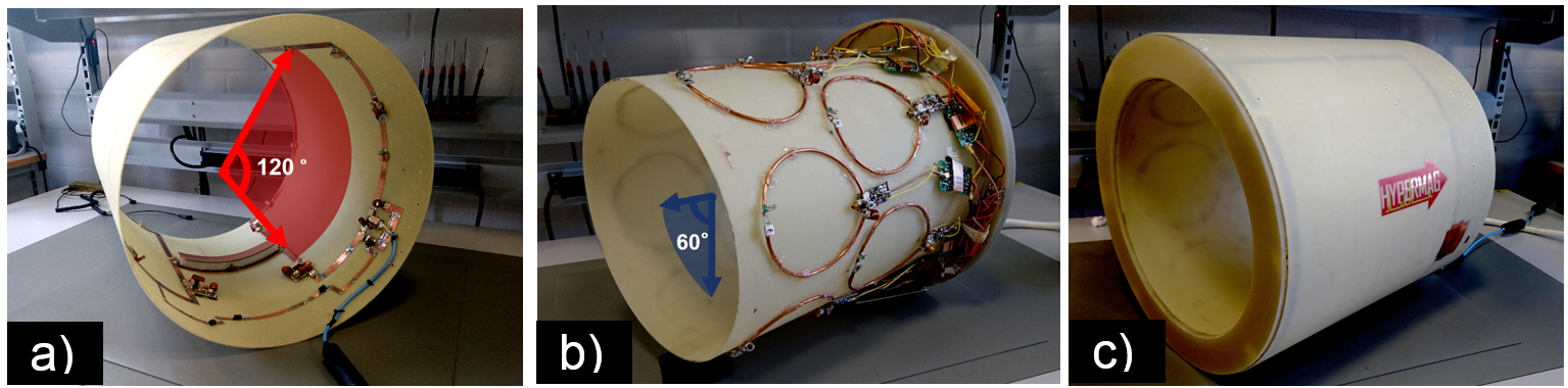
The fabricated coil is shown in Fig. 1. The transmit coil is mounted on the inner part of a 400 mm diameter fiberglass cylinder. The receive array is formed by 12 individual loops of 130 mm diameter, shaped over a 300 mm cylinder. The receive loops are arranged in 2 rows of 6 coils each. This configuration provides a cylindrical FOV of 300 mm diameter and 250 mm long. The coil setup was simulated in CST (Darmstad, Germany) including electronic losses and the decoupling obtained from the mismatched preamplifiers², in order to predict B₁ profiles.

MR Experiments

A reference ¹³C MRS measurement (CSI, 360x360x20 mm³, matrix size = 24 x 24) was performed on a cylindrical ethylene glycol phantom (250 mm diameter, 200 mm long) doped with 17g/L of NaCl, in order to emulate tissue loading. The B₁⁺ profile was calculated using an approach developed earlier³. The B₁^- profile was also evaluated. Additional measurements were done with a similar phantom but without loading (no NaCl). Finally, a ¹³C metabolic imaging experiment of the pig kidney was done on a 40 kg pig, after an injection of hyperpolarized pyruvate. All the MR experiments are done over a single slice, positioned at the center of the front row of coils of the receive array.

Phase Calibration

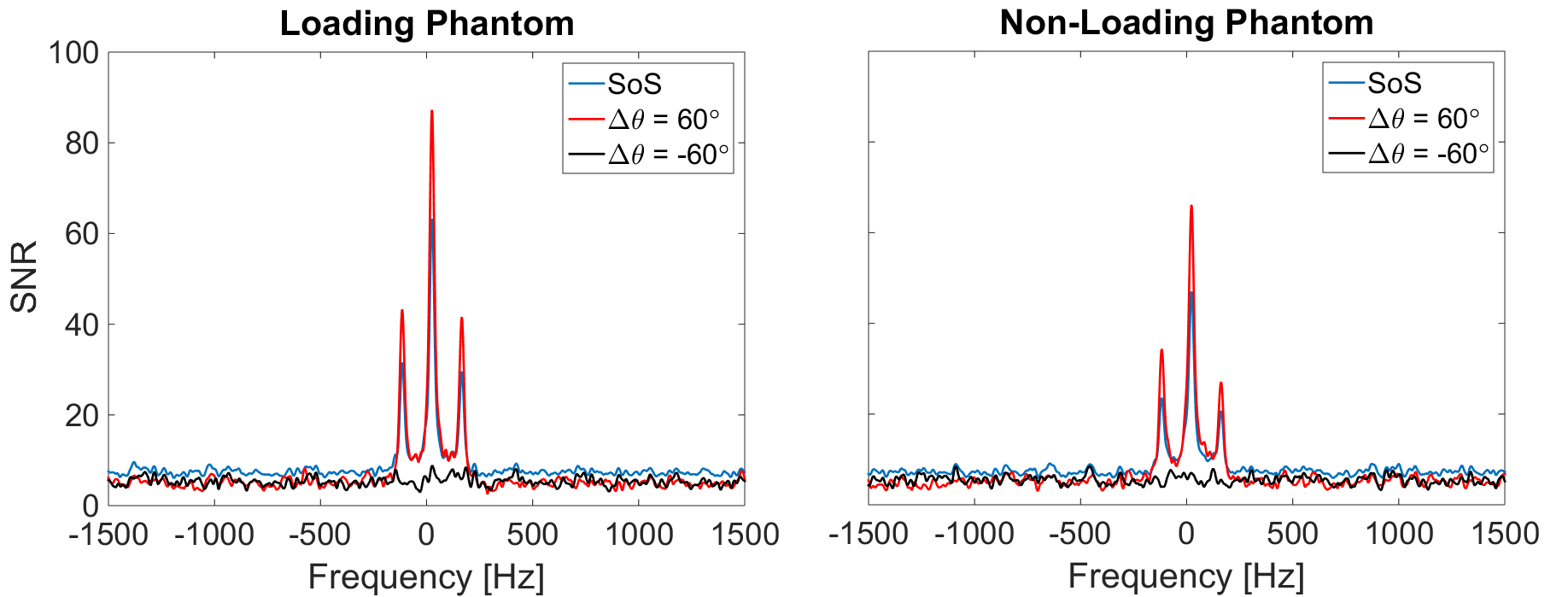
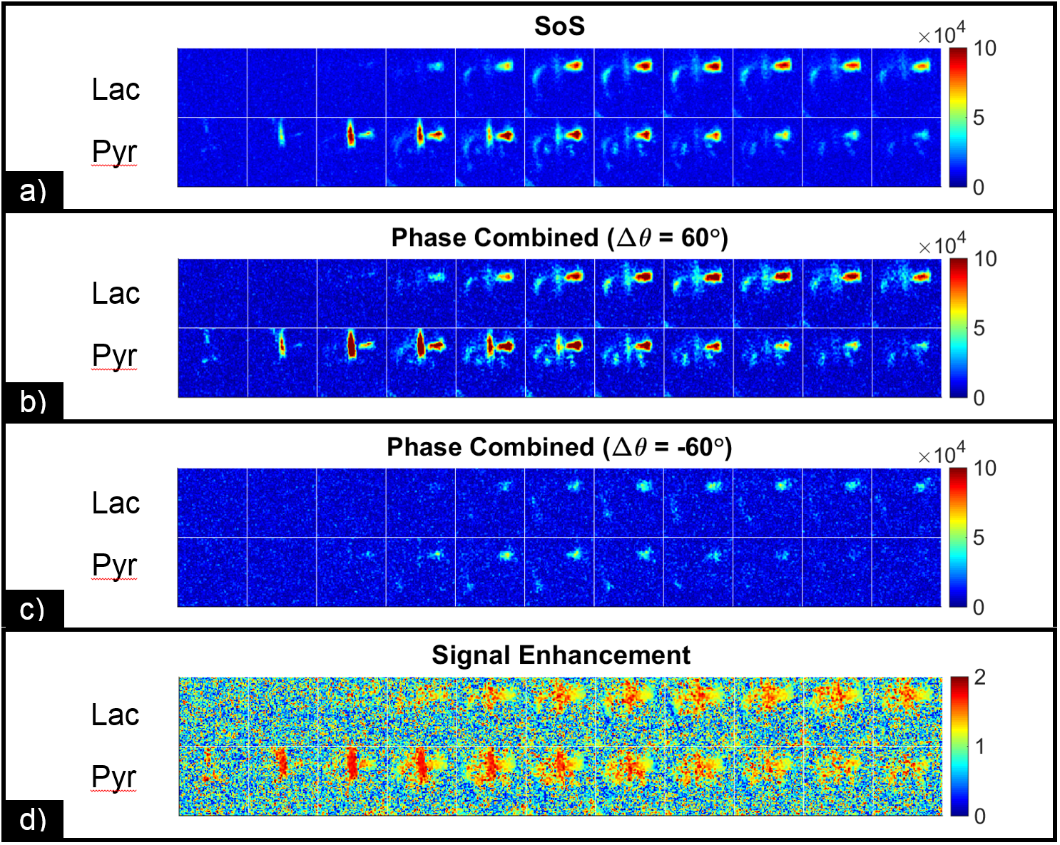
A phase calibration as described in ⁴ was performed from the reference measurement. The phase shifts needed to optimize SNR in a 5x5 voxel region at the center of the coil was calculated using an iterative algorithm. These are the phases that maximize the combined B₁^- (clockwise polarized) field. In an array with circular symmetry, this is equivalent to say that the phase difference between neighboring coils is such that compensates for their geometric separation. For the coil array used here, that means that Δϴ = ϴ_n- ϴ_n-1 = 60°, for each of the 6 elements in a row. For comparison and validation Δϴ = -60° may also be used since this should optimally null the signal (sanity check). The phase shifts (Δϴ = +60° and Δϴ = -60°) calculated from the reference measurement were applied to the other measurements (non-loading phantom and pig), prior to coil combination. The SNR in the central 5x5 voxel region was then compared to SoS. In the coil center, all coils are approximately equally sensitive, and therefore no weighting was applied at this stage.

Results and Discussion

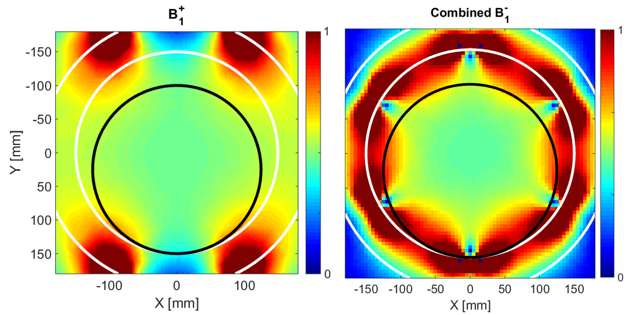
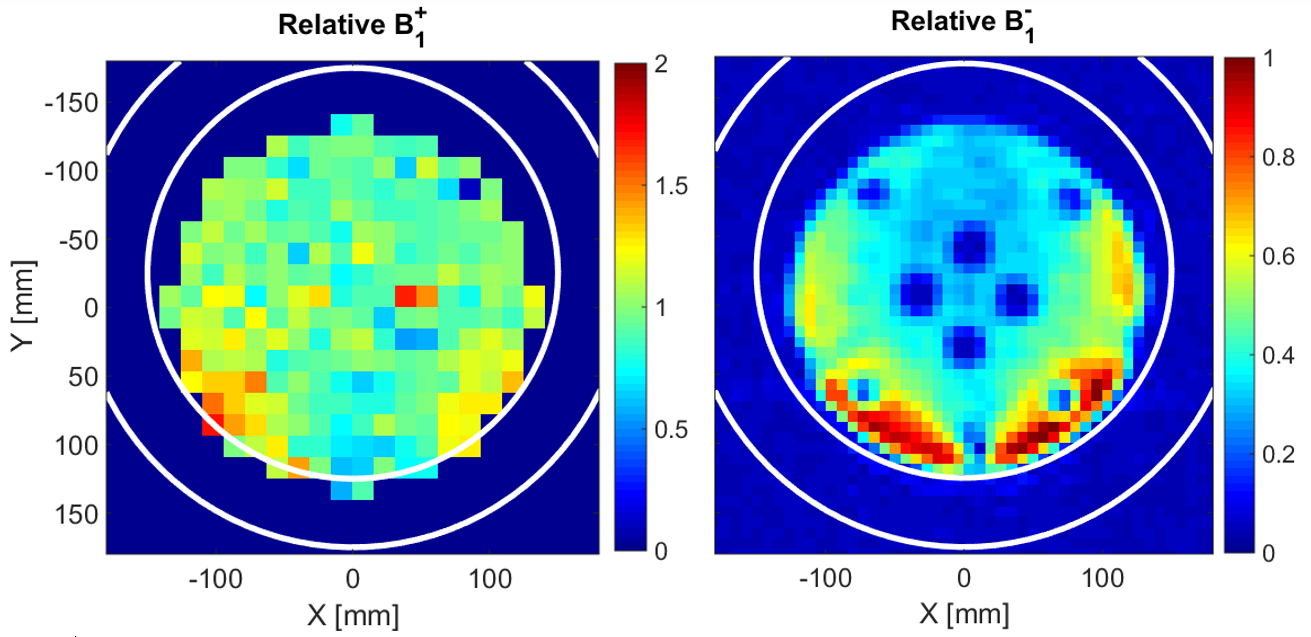
The simulated and measured B₁⁺ and B₁^- profiles are shown in Fig. 2 and Fig. 3 respectively, showing good agreement. The measured SNR is shown in Fig. 4 for the two phantoms (with and without loading), comparing the combination methods. Fig. 5 shows 11 time steps of the kidney metabolic experiment, where the first row corresponds to lactate and the second to pyruvate. A consistent SNR improvement at the center of the coil is obtained when using the phase-calibrated image combination. The phase correction used is the same in all cases, which is consistent with the phase difference introduced by the sample at this frequency being minimal and negligible. Outside of the center where few coils contribute most of the signal, the phasing is less critical, and suboptimal with this simple approach. However, similar localized phase optimization at every position is a simple extension and is expected to improve the SNR in outer regions.

Conclusion

Calibrated coils can be a means to improve MRI in low SNR regions, by both allowing optimal signal combination and improving parallel imaging performance (due to accurate prior information). We show a coil setup that can be phase calibrated to ensure optimal coil combination for ¹³C at 3T. Several loading conditions, including an in-vivo experiment, have been tested and the results indicate that a one-time calibration is enough to fully characterize the coil setup.

Acknowledgements

No acknowledgement found.

References

1. P. B. Roemer, W. A. Edelstein, and C. E. Hayes, “The NMR Phased Array,” MRM, vol. 225, pp. 192–225, 1990.

2. J. D. Sanchez-Heredia, E. S. Szocska Hansen, C. Laustsen, V. Zhurbenko, and J. H. Ardenkjær-Larsen, “Low-Noise Active Decoupling Circuit and its Application to 13C Cryogenic RF Coils at 3T,” TOMOGRAPHY, vol. 3, no. 1, p. 60:66, 2017.

3. R. B. Hansen, “Integrated B1+ Mapping for Hyperpolarized 13C MRI in a Clinical Setup using Multi-Channel Receive Arrays,” ISMRM 2018 Annu. Meet. Exhib., 2018.

4. M. A. Brown, “Time-domain combination of MR spectroscopy data acquired using phased-array coils,” Magn. Reson. Med., vol. 52, no. 5, pp. 1207–1213, Nov. 2004.

Figures

Figure 1. A) Linear ¹³C transmit coil. The coil is formed by two rectangular loops of 419x300 mm (each covering 120° of the coil perimeter), resembling the current pattern of a saddle coil. B) 12-Element receive-only array, where each element has 130 mm of diameter. C) Integrated coil setup, where the two fiberglass cylinders are placed concentrically, so that their relative position is fixed.

Figure 2. Simulated B₁⁺ and B₁^- of the proposed coil (arb. units). The field maps are shown for the XY plane centered at the front row of coils. The overlaid white lines show the coil inner and outer profile. The black line represents the phantom location.

Figure 3. Measured relative B₁⁺ and B₁^- profiles of the fabricated coil. The phantom used includes NaCl doping for the emulation of tissue loading. This measurement is also used to obtain the calibrated phases for optimal coil combination. The overlaid white lines show the coil inner and outer profile.

Figure 4. Measured spectrum at the central 5x5 voxel region for the two different phantoms: loading phantom (left), and non-loading phantom (right). Note that the slightly higher SNR obtained with the loading phantom makes sense, since the coil array is noise matched for a loading situation. Noise was estimated as the standard deviation of a single spectral point at 1000 Hz across all voxels. Note the different noise baselines due to the bias introduced by SoS being removed by the phased summation.

Figure 5. Metabolic imaging of the pig kidney after a hyperpolarized ¹³C Pyruvate injection. 11 time frames of lactate and pyruvate are shown. A) Sum-of-Squares combination. B) Clockwise phase calibrated combination (Δϴ = +60°). C) Counter-clockwise phase calibrated combination (Δϴ = -60°). D) Signal enhancement obtained using the clockwise calibrated phases, compared to SoS.

Proc. Intl. Soc. Mag. Reson. Med. 27 (2019)

1450