1419
Image denoising with deep transfer learning for screening baseball elbow injuries using portable scanners1Institute of Applied Physics, Tsukuba, Japan, 2Comprehensive Human Sciences, Tsukuba, Japan
Synopsis
Portable MRI scanners have the advantages of maximizing clinical availability in remote environments. We have recently developed a portable, elbow scanner installed in a standard-size car. This system allows us to detect early symptoms of baseball elbow in remote places, but it often suffers from the low signal-to-noise ratio in noisy, outdoor environments. Here we proposed a deep-learning based approach, a denoising convolutional neural network with transfer learning, for denoising images of the potable scanner. We verified that the proposed denoising technique improved the quality of noisy images and increased the clinical feasibility of the portable scanner.
INTRODUCTION
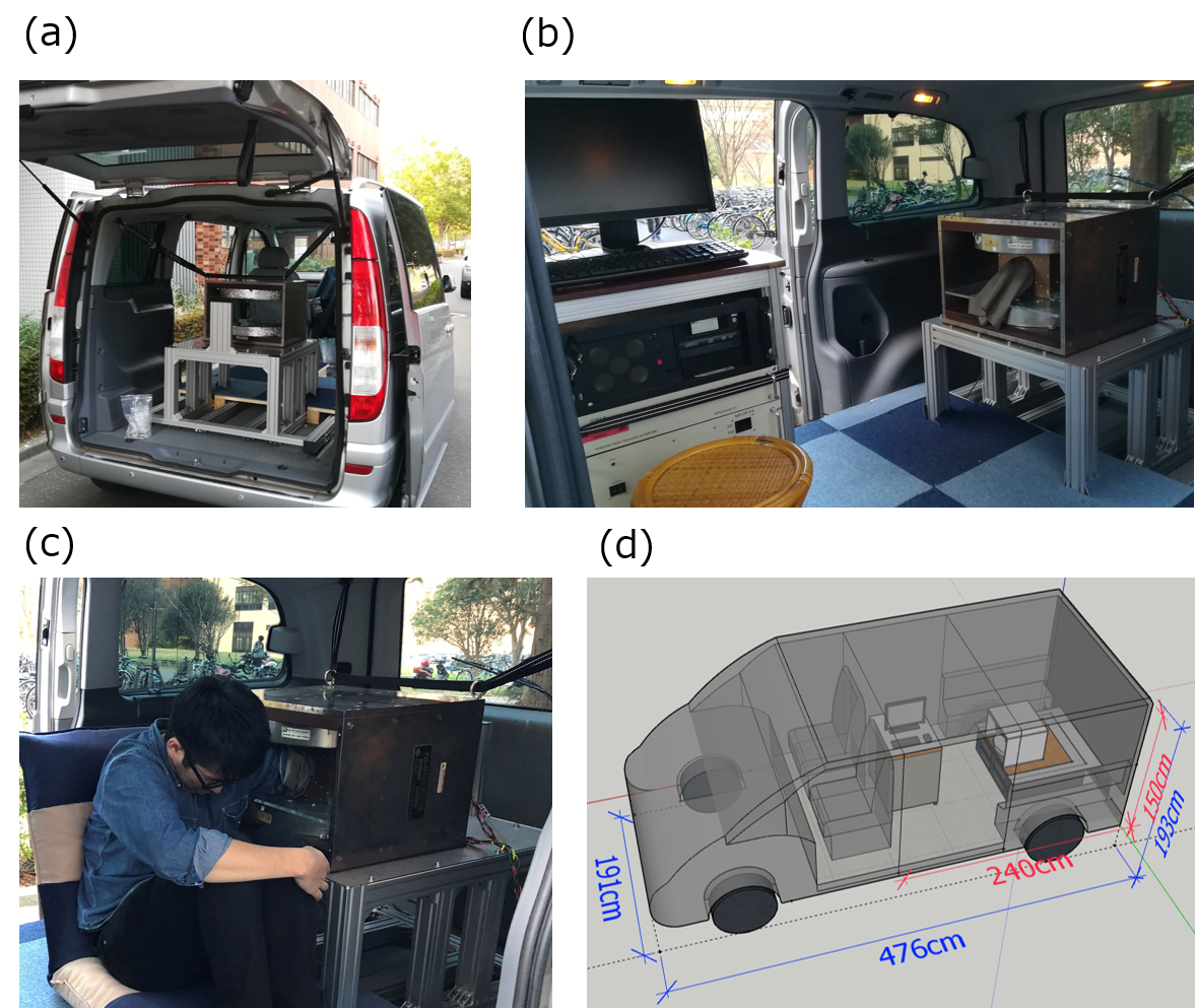
Portable MRI scanners can facilitate medical imaging applications in remote environments, and have potential applications of disease screening of injuries during sport events. We have recently developed a portable, elbow scanner installed in a standard-size vehicle (Fig. 1) [1]. This system has great potential for diagnosing elbow injuries by baseball [2] in baseball grounds, but it often suffers from the low signal-to-noise ratio (SNR) in noisy, outdoor environments. Here we proposed a deep-learning (DL) based, robust approach to improve the image SNR for the potable scanner. The proposed method used a denoising convolutional neural network (DnCNN) [3]. We also used transfer learning because this system has recently been developed and training data for DL was not sufficiently available. The trained networks were used to denoise images of the portable MRI, and the clinical availability of the DL-based denoising was evaluated.METHODS
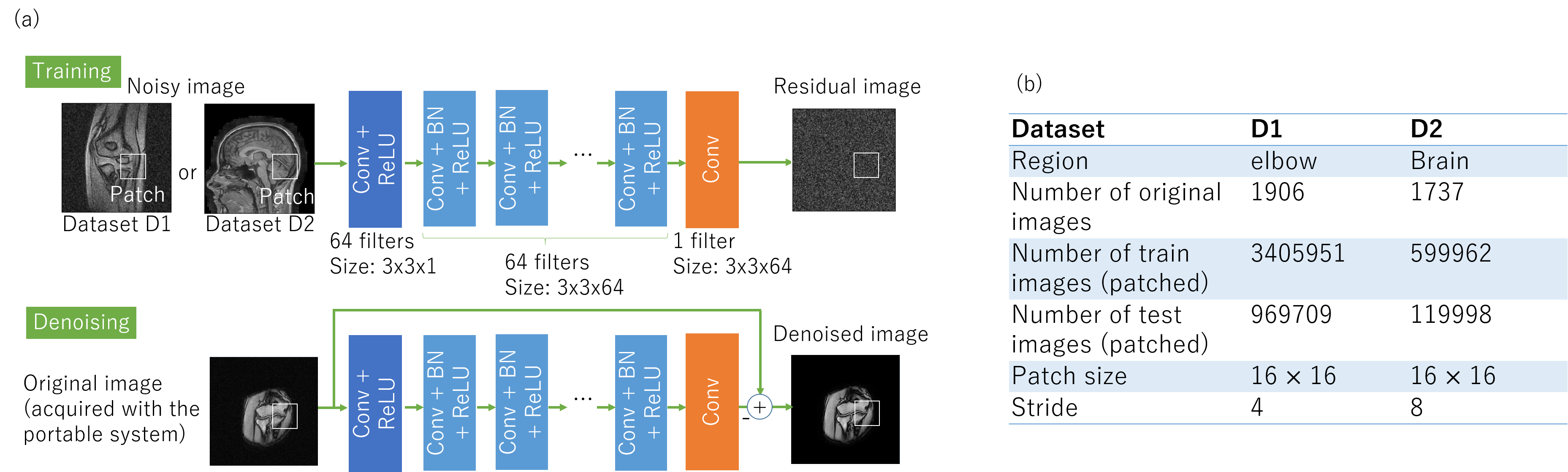
For image denoising, we used a DnCNN with transfer learning (Fig. 2(a)). The DnCNN was designed to predict the residual image. The Rayleigh noises with the variable noise levels (σ = 0.01-0.2) were added to the normalized images. The batch normalization was used to stabilize and enhance the training performance [3]. We set the size of convolutional filers to be 3 x 3 but removed all pooling layers. The network consisted of three types of layers and the network depth was 20.
Two datasets was used to train the network separately (Fig. 2(b)): elbow dataset (D1) acquired using a 0.2 T commercial fixed scanner (C-SCAN; Esaote, Genova, Italy) in the screening procedure of elbow injury [2], and brain dataset (D2) of T1-weighted, T2-weighted, PD-weighted images downloaded from the website [4]. The D1 images were acquired with a coronal gradient-echo sequence (TR = 500 ms, TR = 18 ms, slice thickness = 3 mm, matrix size = 256 x 192, FOV = 180 x 180 mm, 10 slices).
We used Adam algorithm and trained 50 epochs. The learning rate was decayed exponentially from 0.1 to 0.0001. We used the Keras package [5], and all the experiments were performed in the python environment. It took about one hour to train the model on GPU (NVIDIA GTX 1080).
The trained networks were transferred to denoise elbow images (54 images; 9 subjects) acquired using the portable scanner with a 0.2 T permanent magnet [1] (200 kg; 16 cm gap; 44 cm x 50 cm x 36 cm; Imaging volume = 10 cm DSV). These images were acquire with the same sequence parameters as those of the D1 dataset. For denosing, the patch size = 16 × 16 and stride = 1. The patched images were averaged, synthesized, and restored to the same size as the original image.
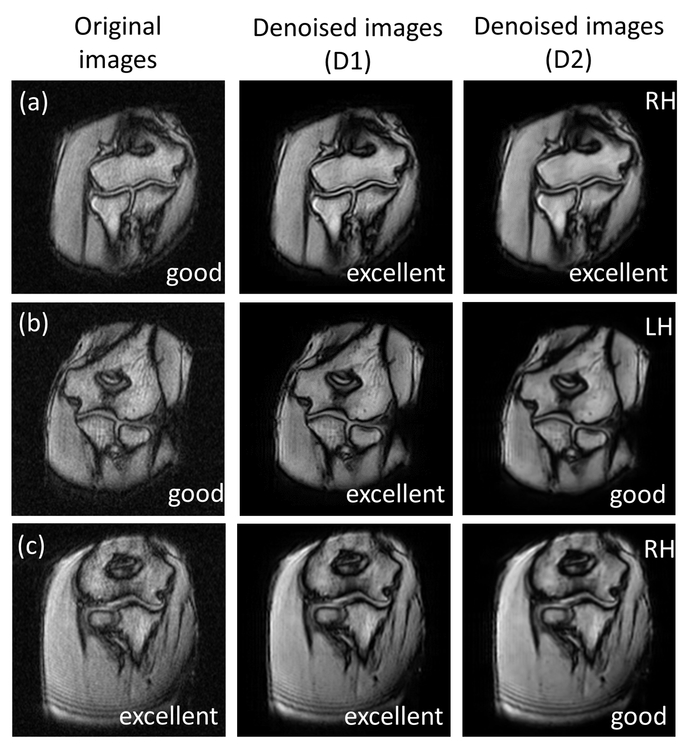
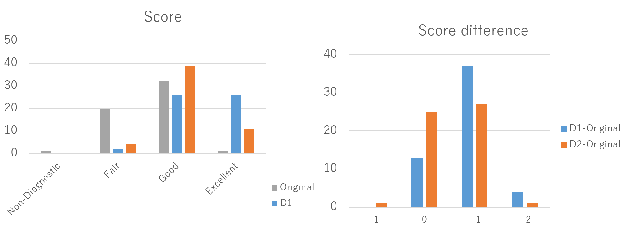
The image quality of the original and denoised images was graded by a radiologist (18 years of experience in musculoskeletal radiology) on a 4-point scale: 1 = nondiagnostic, 2 = fair, 3 = good, and 4 = excellent.
RESULTS AND DISCUSSION
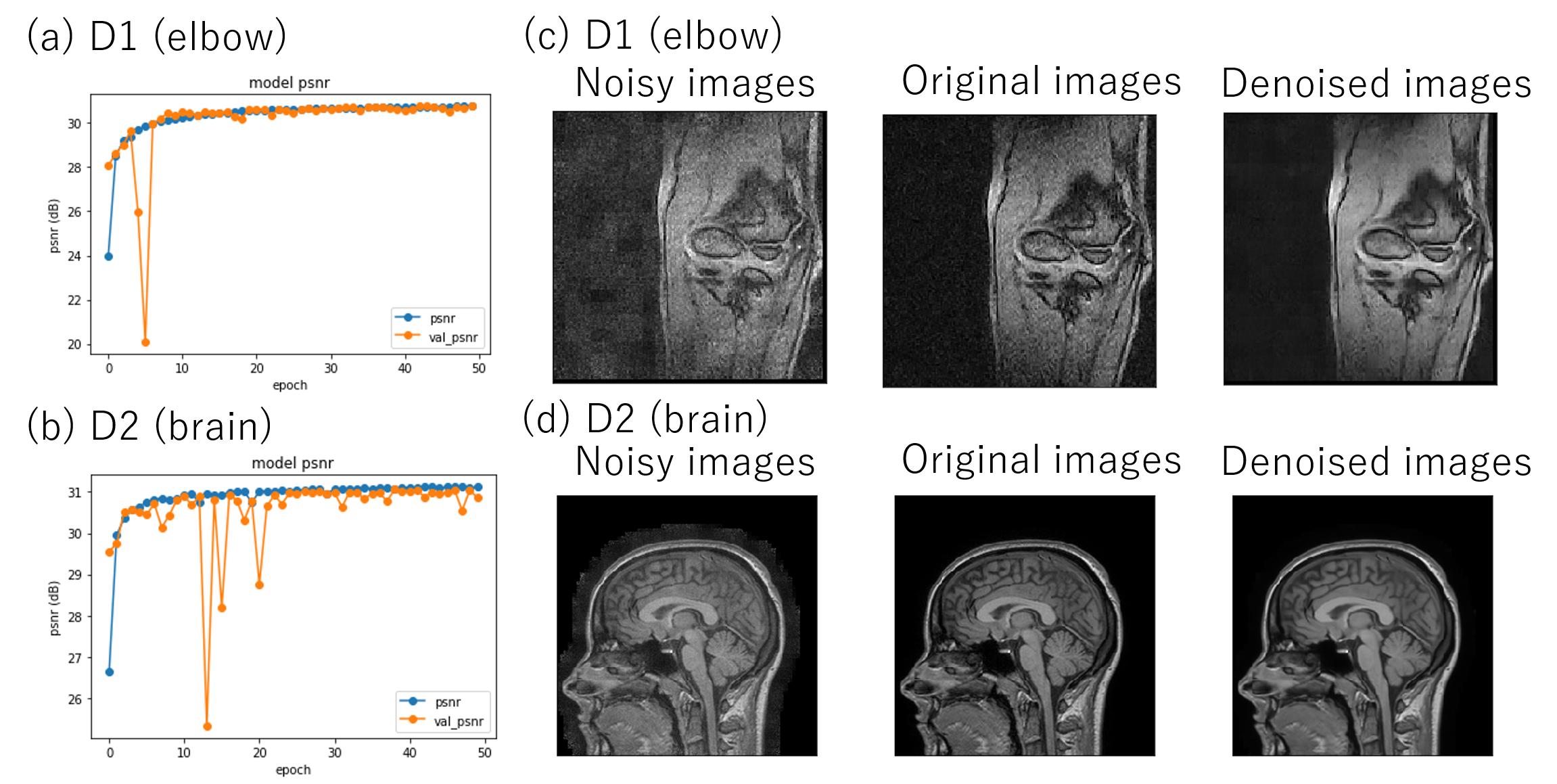
Figure 3 shows the results of network training using different dataset D1 and D2, which showed the stable training process and high denoising performance in both cases. Figures 4 and 5 show the denoising results using the learned networks D1 and D2. For both D1 and D2-based denosing, the denoised images mostly had the improved quality than the original ones (Fig. 4(a)), and the scores were high compared with the original images (Fig. 5). In some cases, only the D1-based denoisiging gave the better results (Fig. 4(b)). In other cases, the D2-based denoising degraded the image quality (Fig. 4(c)). According to the rater’s comments for denoising results, the D1-based denoising was better than the D2-based denoising in most cases. This is possibly because the D1 dataset had the similar image contrast with the denoised images. The rater also commented that the D1-based denoising retained the detailed, anatomical information in most cases, and that the D2-based denosing erased or blurred the tissues in some cases. These results indicate the proposed denosing method improved diagnostic feasibility and clinical reliability.CONCLUSION
In this study, we proposed the robust, learning-based denosing technique that can improve the quality of noisy images of the portable scanner, and improve the diagnostic feasibility and clinical reliability.Acknowledgements
No acknowledgement found.References
[1] K. Tanabe et al., “Development of a small-car mountable MRI system for human extremities using a 0.2 T permanent magnet,” Proc. Intl. Soc. Mag. Reson. Med. 26, 4423, (2018).
[2] Y. Okamoto et al., Incidence of elbow injuries in adolescent baseball players: screening by a low field magnetic resonance imaging system specialized for small joints, Jpn J Radiol, 34: 300-6 (2016).
[3] K. Zhang et al. Beyond a Gaussian Denoiser: Residual Learning of Deep CNN for Image Denoising, IEEE Trans Image Processing, 26: 3142-3155 (2-17).
[4] https://brain-development.org/ixi-dataset/
[5] Chollet et al (2015), GitHub repository, https://github.com/fchollet/keras
Figures