Synopsis

The relationship between image biomarkers in structural MRI and knee osteoarthritis pain progression is investigated. A Bayesian Gaussian mixture model is selected to identify the distinct knee pain trajectories among subjects in the dataset from the Osteoarthritis Initiative. Deep learning is employed to predict the probability of an individual’s pain curve cluster membership using the 3D structural MRI. Utilizing the strength of the model-based approach, the pain curves are simulated from the GMM posterior probabilities and the weights learned to evaluate the 3D DenseNet’s performance.

Introduction

Methods

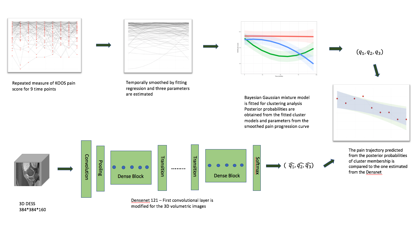
Datasets: A total of 4,796 subjects’ repeated measures of KOOS pain score4 for both knees over 10-year study were obtained from the Osteoarthritis Initiative. 3D Double Echo Steady State (DESS) images of knee for the subjects at baseline were used for the image biomarker discovery. Parameters of sagittal 3D sequence are: TR/TE 16.2/4.7 ms, FOV=14cm, matrix size=307x348, bandwidth=248 Hz/pixel, image resolutions =0.346x0.346x0.7 mm. The data processing overall pipeline is described in Figure 1.

Modeling pain trajectory: We temporally smoothed individual’s pain curve by fitting a regression model using the orthogonal polynomials of degree 1 and 2 as the basis in order to reduce the inherent noise in the dataset and to handle missing data. The estimated parameters were standardized to be used as input into the Bayesian Gaussian mixture model for clustering analysis. Silhouette approach was used to choose the optimal model that captures the distinct pain patterns best. The parameters from regression were re-fitted against the selected Gaussian mixture model’s means to obtain the posterior probabilities of each pain curve that describe the cluster membership. A total of 24 candidate models of varying number of components (2, 3, 4, 5, 6) and different types of covariance (full, tied, diagonal, spherical) were optimized using the expectation-maximization algorithm.

Deep learning architecture and training details: Our network is a 3D extension of the DenseNet 121 architecture5,6. The training dataset images were augmented by randomly applying image operations including horizon flipping, translation (up to 18 pixels vertically and horizontally), and rotation ([-15, +15] degrees). In doing so, the images those are most likely be the rare classes were boosted by applying the transformation 9 times per image to alleviate the effect of class imbalance. The weights were initialized using the He initialization. The network was trained to learn the posterior probabilities of pain trajectory membership. Mean squared error function was used as the loss function for regression. Additional details on hypermeters choice are included in Figure 2.

Results

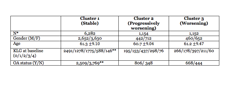
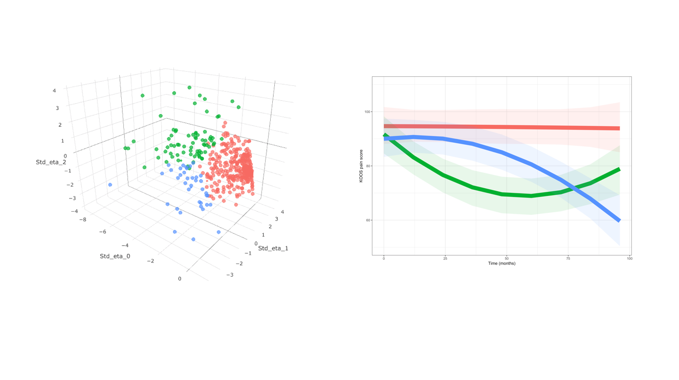
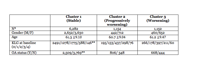
Pain trajectory clustering analysis: The Gaussian Mixture of three components with tied covariance, which had the highest mean silhouette score, was selected as the optimal clustering model. The clustering analysis based on the GMM model identified three distinct pain trajectories: stable, worsening, progressively worsening (Figure 3). Demographic and clinical profiles for each of clusters are reported in Figure 4. The distribution of age and gender were very similar across the clusters, while the Kellgren-Lawrence grades and OA status were more severe in the progressively worsening cluster.

Training results: The mean squared error scores were 0.0148, 0.1556, 0.1549 for training(n=5,470), validation(n=1,368), and test(n=1,710) set, respectively. The mean absolute error scores were 0.0174, 0.1661, 0.1654 for training, validation, and test set, respectively. The accuracy score, which measures whether the network correctly predicts the most probable clusters, were 0.9853, 0.8041, 0.7830 for training, validation, and test set, respectively.

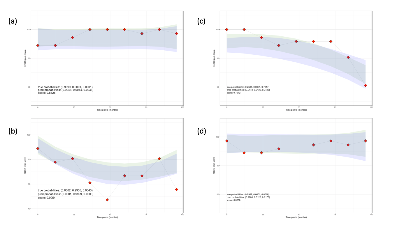
Pain curve prediction: We evaluated the model’s performance by comparing the simulated pain trajectories with the posterior probabilities of fitted GMM to the ones with the posterior probabilities the deep learning learned from MRI images. We simulated 1,000 sets of a random sample to obtain the confidence intervals and measured the overlap over the union of the intervals. The results were 0.8489, 0.5935, 0.5991 for the train, validation, test set, respectively. Figure 4 shows some examples of DL performed well in predicting future pain.

Discussion

We built a deep learning model that relates automatic learned MRI imaging biomarkers to temporal information of the knee pain. With our design we can provide, not only the point estimate but also the uncertainty incorporated into the problem. As the analysis was focused on the relationship between image biomarker and pain, other clinical and demographic patient information was not examined. We plan to expand our model to consider other factors that can impact the OA pain management.

Acknowledgements

References

[1] Halilaj E, et el., Modeling and predicting osteoarthritis progression: data from the osteoarthritis initiative, Osteoarthritis Cartilage, doi: 10.1016/j.joca.2018.08.003

[2] Nicholls E, et el., Pain trajectory groups in persons with, or at high risk of, knee osteoarthritis: findings from the Knee Clinical Assessment Study and the Osteoarthritis Initiative, Osteoarthritis Cartilage, doi:10.1016/j.joca2014.09.026

[3] Losina E, Collins JE. Forecasting the future pain in hip OA: can we rely on pain trajectories? Osteoarthritis Cartilage, doi:10.1016/j.joca.2016.01.989

[4] Roos EM, Lohmander LS. Knee injury and Osteoarthritis Outcome Score (KOOS): from joint injury to osteoarthritis. Health Qual Life Outcomes 2003;1:64.

[5]Huang G, et el., Densely connected convolutional networks, arXiv preprint arXiv:1608.06993, 2016a

[6]Hara K, et el., "Can Spatiotemporal 3D CNNs Retrace the History of 2D CNNs and ImageNet?", Proceedings of the IEEE Conference on Computer Vision and Pattern Recognition, pp. 6546-6555, 2018.