1404
Assessing the performance of knee meniscus segmentation with deep convolutional neural networks in 3D ultrashort echo time (UTE) Cones MR imaging1Department of Radiology, University of California, San Diego, CA, United States, 2Radiology Service, VA San Diego Healthcare System, San Diego, CA, United States, 3Departments of Orthopedic Surgery and Bioengineering, University of California, San Diego, CA, United States
Synopsis
Automatic segmentation of the knee menisci would facilitate quantitative and morphological evaluation in diseases such as osteoarthritis. We propose a deep convolutional neural network for the segmentation of 3D UTE-Cones Adiabatic T1ρ-weighted volumes of the meniscus. To show the usefulness of the proposed method, we developed the models using regions of interests provided by two radiologists. The method produced strong Dice scores and consistent results with respect to meniscus volume measurement. The inter-observer agreement between the models and the radiologists was very similar to that of the radiologists alone.
Introduction
Osteoarthritis (OA) is the most common form of arthritis in the knee1. The meniscus plays a key role in the initiation and progress of OA. However, it has a short T2 and demonstrates low signal on conventional MR sequences. The 3D ultrashort echo time Cones Adiabatic T1ρ (3D UTE-Cones-AdiabT1ρ) sequence provides high signal and quantitative measurement of AdiabT1ρ2, which may provide more accurate evaluation of meniscus degeneration. Manual segmentation of the menisci, however, is time consuming and requires experienced readers3. In this work, we proposed a fully automated segmentation algorithm of the menisci based on a U-Net deep convolutional neural network (CNN)4. The performance of the proposed approach was evaluated using manual segmentation provided by two radiologists. Additionally, the inter-observer agreement was studied.Methods
A total of 67 human subjects was recruited for 3D UTE-Cones-AdiabT1ρ imaging on a 3T scanner (MR750, GE Healthcare). Informed consent was obtained from all subjects in accordance with guidelines of the institutional review board. The 3D UTE-Cones-AdiabT1r sequence employed the following imaging parameters: TR=500 ms; FOV=15×15×10.8 cm3; bandwidth=166 kHz; FA=10°; matrix=256×256×36; number of paired adiabatic inversion pulses NIR=0, 2, 4, 6, 8, 12 and 16 each with a scan time of 2 min 34 sec2. Regions of interests (ROIs) indicating the menisci were outlined by two experienced radiologists (22 and 11 years of experience, respectively). The dataset was divided into training, validation and test sets with a 47/10/10 split. All images were preprocessed with the local contrast normalization algorithm. Next, the training set was augmented by rotating and horizontal flipping to generate 4152 labeled 2D images. To improve the CNN performance, additional batch normalization and drop-out layers were employed. In comparison to other studies5-7, we trained our model to simultaneously minimize the weighted binary cross entropy loss and maximize the Dice coefficient. To show the usefulness and the robustness of our approach, we separately compared the test set performance of the networks trained using the ROIs provided by the radiologists. CNNs were developed using the ROIs outlined by the first and second radiologists (CNN1 and CNN2, respectively).Results and Discussion
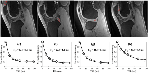
Representative 3D UTE-Cones-AdiabT1r images of a 23y old volunteer are shown in Figure 1. The meniscus is depicted with high resolution and SNR, with excellent fitting demonstrating a T1r of 21.5±1.1ms.
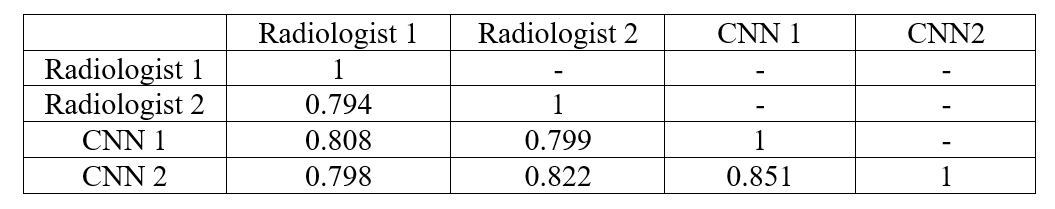
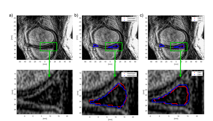
The average Dice score between the ROIs generated by the radiologists was equal to 0.794, indicating good inter-observer agreement. Both CNN models produced strong Dice coefficients equal to 0.808 and 0.822 for CNN1 and CNN2, respectively. Additionally, the Dice score between the ROIs calculated using both CNNs was equal to 0.851. The Dice score between the first radiologist and CNN2 (developed using the second radiologist’s ROIs) was equal to 0.798. Similarly, in the case of the second radiologist and CNN1, the Dice score was equal to 0.799. The agreement between the radiologists was the same as between the radiologist and the deep learning model developed using ROIs provided by another radiologist. Moreover, significantly higher agreement between the CNN models than between the radiologists suggest that the networks successfully generalized how to segment the menisci based on image pixel intensities. Results are summarized in Table 1. Both deep learning models were excellent at detecting menisci pixels with the area under the receiver operating characteristic curve higher than 0.94. Figure 2 shows a comparison between the manual segmentation and the automatic segmentation obtained using the CNNs. While the detection of the menisci by the CNNs was robust, achieving perfect overlapping between the ROI provided by the radiologist and that calculated by the model was difficult due to low visibility of the menisci borders. We found that, for each model, the Dice score was correlated with the size of meniscus ROI generated by manual segmentation. This indicates that the Dice coefficient may not be a good predictor of the segmentation performance if the meniscus area is small.
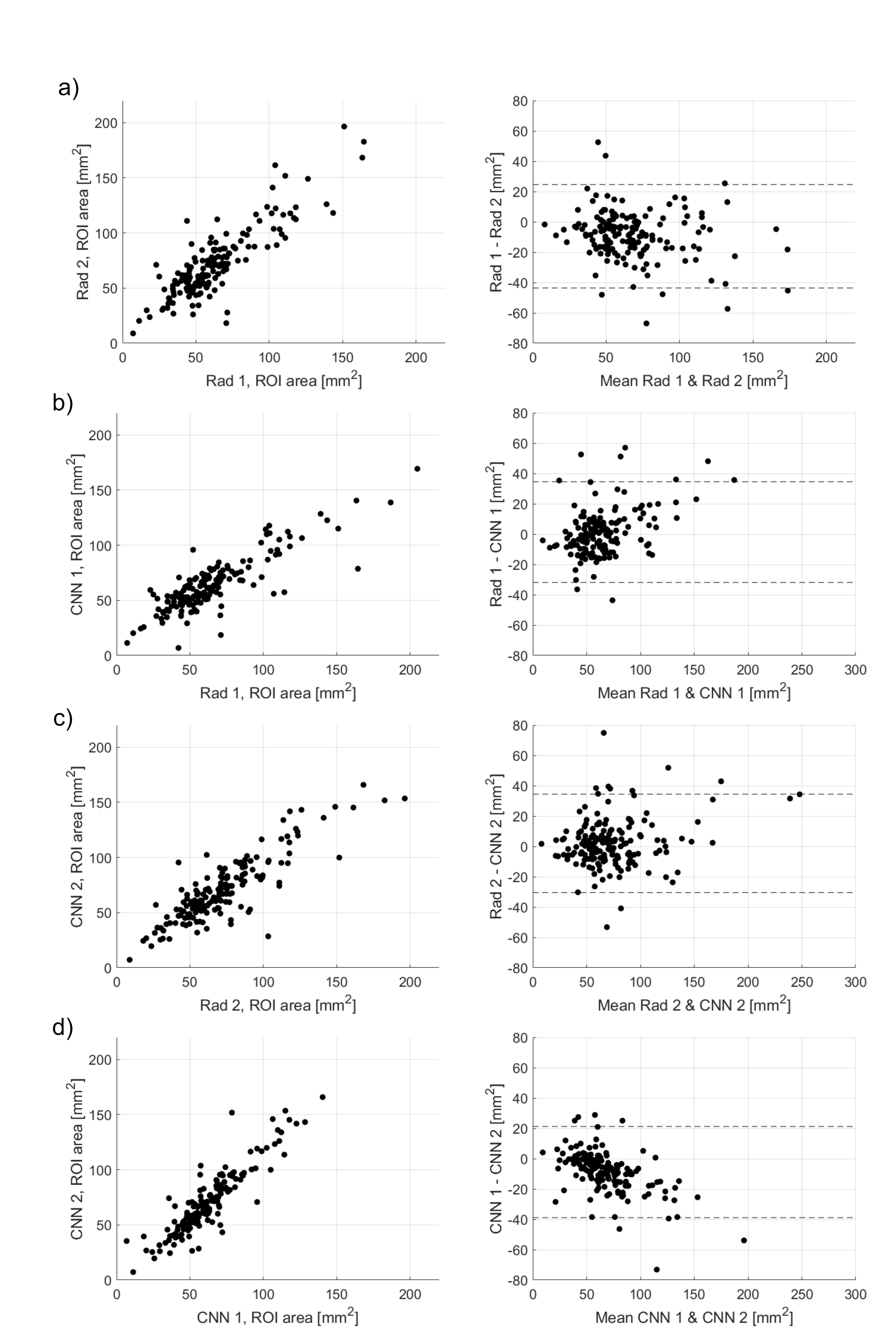
Figure 3 shows the consistency of menisci measurements between the radiologists and the models. The Spearman’s rank correlation coefficient between the areas determined using radiologists’ ROIs were equal to 0.799. Again, higher agreement was obtained in the case of the ROIs calculated by the CNNs, 0.883. Bland-Altman plots in Figure 3 indicate that the area estimates produced by the radiologists and the models were consistent.
Conclusion
We proposed an efficient method for meniscus segmentation, which can be used to provide morphological and quantitative data related to meniscus shape and volume (and potentially AdiabaticT1ρ mapping). Presented results suggest that the CNNs achieve performance similar to that obtained by the radiologists.Acknowledgements
The authors acknowledge grant support from the VA Rehabilitation Research & Development Service (I01RX002604), VA Clinical Science Research & Development Service (I01CX001388) and National Institutes of Health (R01AR062581).References
- Loeser RF, Goldring SR, Scanzello CR, Goldring MB. Osteoarthritis: a disease of the joint as an organ. Arthritis Rheum. 2012;64(6):1697-707.
- Ma YJ, Carl M, Searleman A, Lu X, Chang EY, Du J. 3D adiabatic T1rho prepared ultrashort echo time cones sequence for whole knee imaging. Magnetic resonance in medicine 2018;80(4):1429-1439.
- Eckstein F, Kwoh CK, Link TM, OAI investigators. Imaging research results from the Osteoarthritis Initiative (OAI): a review and lessons learned 10 years after start of enrolment. Ann Rheum Dis. 2014;73:1289-1300.
- Ronneberger, O, Fischer P, Brox T. U-net: Convolutional networks for biomedical image segmentation. In International Conference on Medical image computing and computer-assisted intervention. 2015;234-241. Springer, Cham.
- Norman B, Pedoia, V, Majumdar S. Use of 2D U-Net Convolutional Neural Networks for Automated Cartilage and Meniscus Segmentation of Knee MR Imaging Data to Determine Relaxometry and Morphometry. Radiology, 2018;172322.
- Tack A, Mukhopadhyay A, Zachow S. Knee menisci segmentation using convolutional neural networks: data from the Osteoarthritis Initiative. Osteoarthritis and cartilage, 2018;26:680-688.
- Zhou Z, Zhao G, Kijowski R, Liu F. Deep convolutional neural network for segmentation of knee joint anatomy. Magn Reson Med. 2018;80:2759-2770.
Figures