Synopsis

Manual annotation of muscle is still one of the most time-consuming steps in skeletal muscle MRI research. In this study we have investigated three aspects of automated muscle annotation using deep convolutional networks. First, we directly compare five different network architectures. Second, we compare the effect of providing various input data all based on Dixon imaging. Third, we investigate the effect of the amount of training data provided to the network. In summary we found that UNet-like convolutional networks allow for accurate and precise annotation of calf muscle in 2D and 3D and that the data provided is the strongest predictor of success.

Introduction

Methods

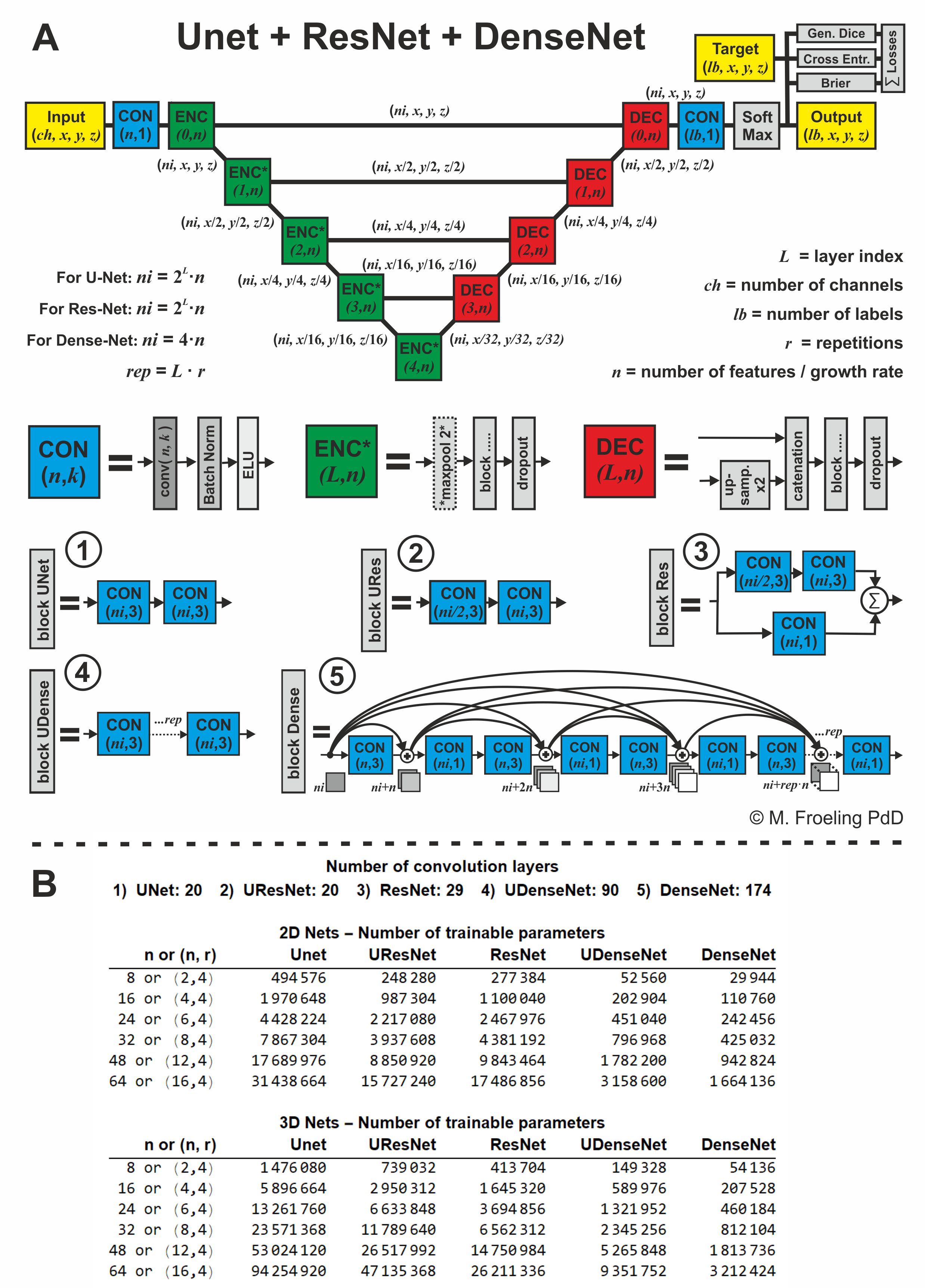
Five different 2D and 3D segmentation networks were designed, i.e. UNet, UResNet, ResNet, UDenseNet, DenseNet. The networks have varying numbers of convolution layers (depth) and trainable parameters, and are based on popular architectures in the literature (5–7) (see Fig. 1). To improve the flow of gradients through backpropagation ResNet and DenseNet have skip connections. All networks were implemented in Mathematica 11 using a toolkit based upon MX-Net (github.com/mfroeling/UNET). As a loss function, we used a linear combination of a cross entropy, a soft Dice and a Brier loss layer (8–11).

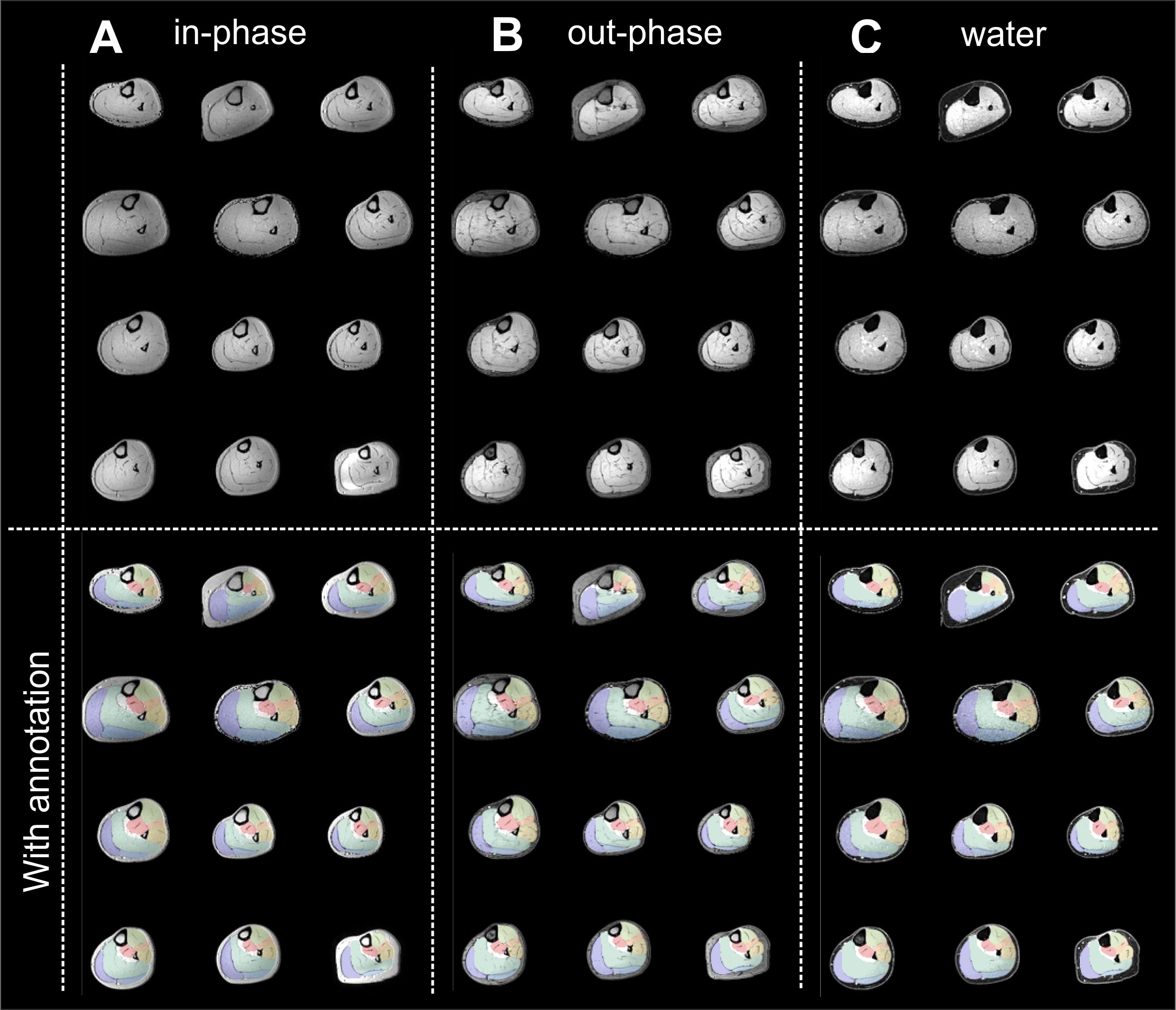
MRI Dixon data of the calf was acquired bilaterally in 59 subjects using a 4-point Dixon scan (TE 2.6/3.36/4.12/4.88 ms, TR 210 ms, 1.5x1.5x3mm³). Seven muscles were manually annotated in all legs by an expert and checked by two other experts. Both the left and right leg were cropped to a FOV of 32x112x112 voxels after which the left leg was mirrored to match the right. Therefore, in total 118 annotated calfs were available for training, validation and testing (see Fig. 2). In addition to varying the network architecture, we varied the input information to the network. This was either the in-phase image, the out-phase image, the water image, or a three-channel concatenation of these three images.

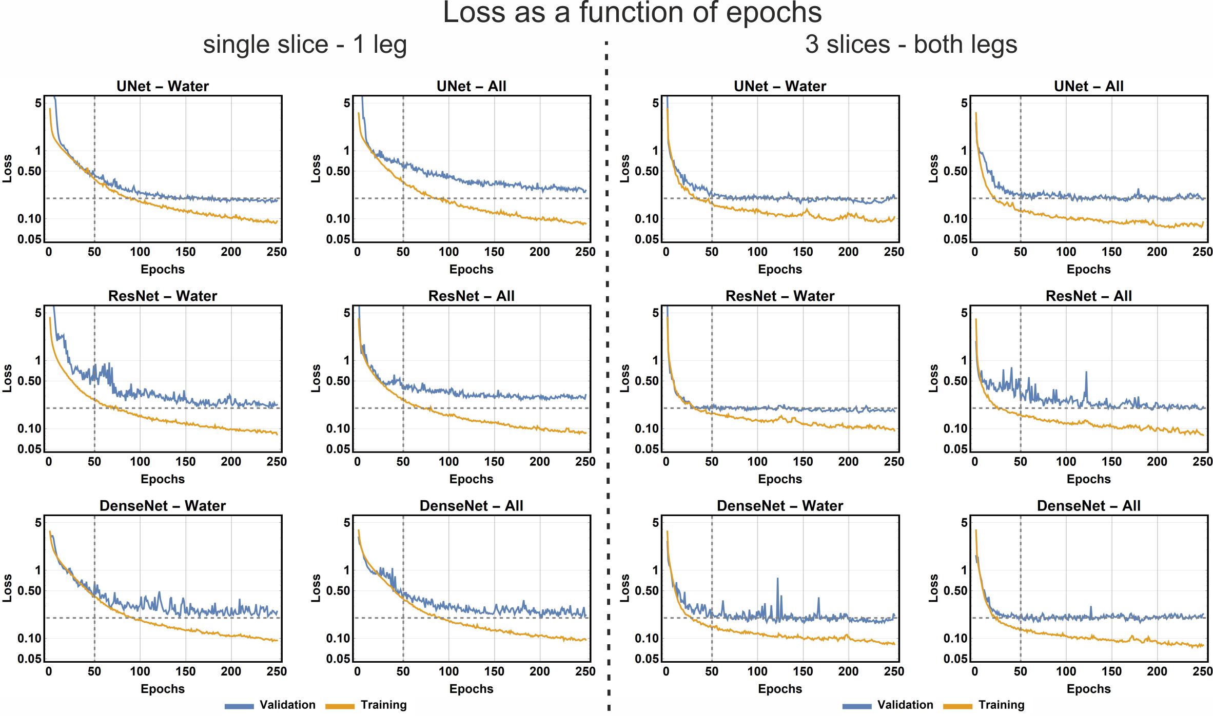
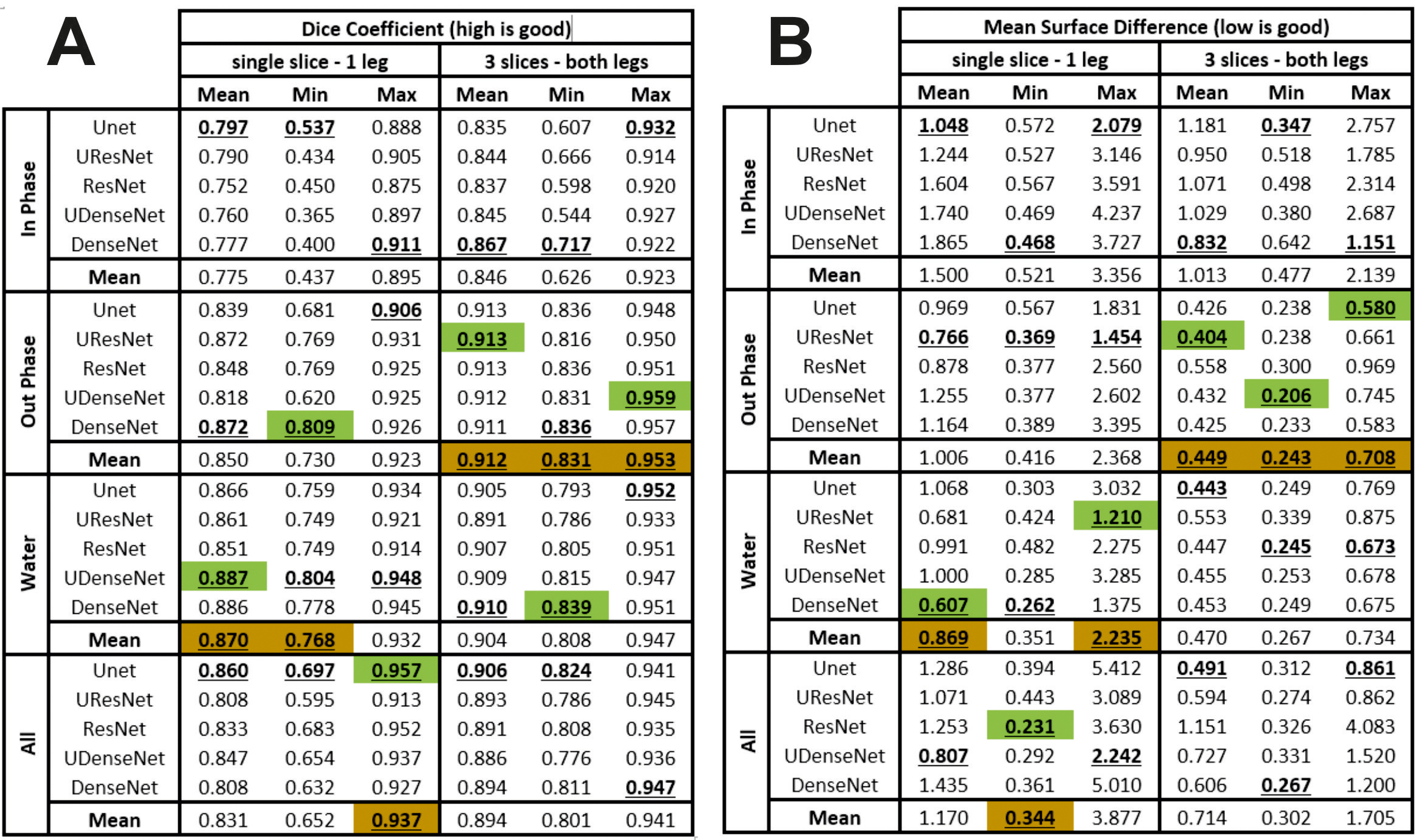
To evaluate the effect of the amount of training data, networks were either trained using only the middle slice of the left leg (59 slices, SET1) or three equidistant slices of both legs (118x3 = 354 slices, SET2). The data was split into a training (80%), validation (15%) and testing (5%) sets. All training was performed with a batch size of 24 and 250 epochs using a NVIDIA Titan Xp graphics card. The number of feature maps in the first layer was always 48, by setting n = 48 or (n,r) = (12,4) (see Fig. 1B). Results were evaluated using the Dice and MSD (in voxels) scores.

Results

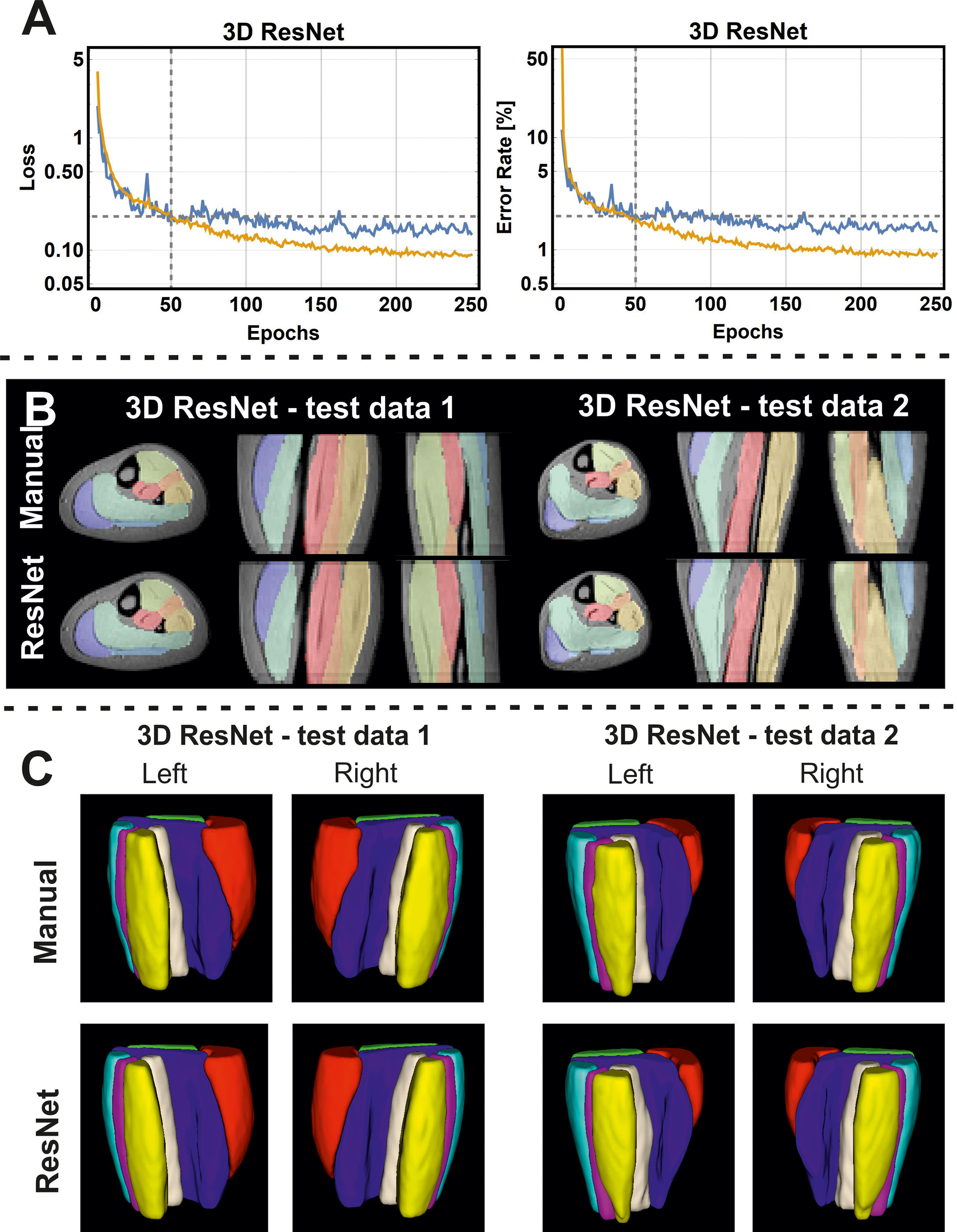
Examples of the loss and error-rate as a function of epochs is shown in Fig 3. Overall the network architecture and the amount of data had little influence on the training results (see Fig. 4). Including more data in a network with more convolution layers in general allowed for slightly faster convergence, but always resulted in similar Dice and MSD values. However, we found that the kind of input data used by the network had a large effect on the training results. In-phase images performed considerably worse than out-phase or water images. When all three images were combined the results were worse than training on the water of out-phase images alone.

We found that the best performing 2D network was a ResNet network, and consequently also trained a 3D variant of this model with identical hyperparameter settings. For this model, segmentation using the out-phase data as input resulted in a mean Dice of 0.901 (range 0.815 to 0.949) and a mean MSD of 0.408 (range 0.200 to 0.677) voxel on the training set (5% of scans) (see Fig. 5).

Discussion and conclusion

Our results showed that the kind of data provided to a UNet-like convolutional network for calf segmentation is a more important factor than the exact layout of individual building blocks. The in-phase data has poor contrast between water and fat and does not clearly show tendons and aponeuroses and water and out-phase images are preferred. Nevertheless, this may be due to a bias in the manual segmentations, which are typically performed on out-phase images.

In summary we found that UNet-like convolutional networks allow for accurate and precise annotation of calf muscle in 2D and 3D and that the data provided is the strongest predictor of success.

Acknowledgements

References

1. Fouré A, Ogier AC, Le Troter A, et al.: Diffusion Properties and 3D Architecture of Human Lower Leg Muscles Assessed with Ultra-High-Field-Strength Diffusion-Tensor MR Imaging and Tractography: Reproducibility and Sensitivity to Sex Difference and Intramuscular Variability. Radiology 2018; 287:592–607.

2. Fischer M, Schwartz M, Yang B, Schick F: Random Forest based Calf Muscle Segmentation from MR data incorporating Prior Information. In Proc 26rd Annu Meet ISMRM, Paris, Fr; 2018:2840.

3. Snezhko E, Azzabou N, Baudin P-Y, Carlier PG: Convolutional neural network segmentation of skeletal muscle NMR images. .

4. Konda A, Crump K, Podlisny D, et al.: Fully automatic segmentation of all lower body muscles from high resolution MRI using a two-step DCNN model. In Proc 26rd Annu Meet ISMRM, Paris, Fr; 2018:1398.

5. Huang G, Liu Z, van der Maaten L, Weinberger KQ: Densely Connected Convolutional Networks. 2016.

6. He K, Zhang X, Ren S, Sun J: Deep Residual Learning for Image Recognition. 2015. 7. Ronneberger O, Fischer P, Brox T: U-Net: Convolutional Networks for Biomedical Image Segmentation. 2015.

8. Milletari F, Navab N, Ahmadi S-A: V-Net: Fully Convolutional Neural Networks for Volumetric Medical Image Segmentation. 2016.

9. Mannor S, Peleg D, Rubinstein R: The cross entropy method for classification. In Proc 22nd Int Conf Mach Learn - ICML ’05. New York, New York, USA: ACM Press; 2005:561–568.

10. Young RMB: Decomposition of the Brier score for weighted forecast-verification pairs. Q J R Meteorol Soc 2010; 136:

11. Sudre CH, Li W, Vercauteren T, Ourselin S, Cardoso MJ: Generalised Dice overlap as a deep learning loss function for highly unbalanced segmentations. 2017.