Synopsis

Water proton $$$R_2$$$ relaxation in cartilage at 3T contains both an isotropic and an anisotropic contributions, with the latter being more sensitive to degenerative changes. A composite relaxation ($$$R_2-R_{1ρ}$$$) mapping could be used to separate two contributions; however, its lengthy protocol had prevented it from being adopted in clinical applications. Here, we propose an efficient alternative based on a single T2W sagittal image to isolate an anisotropic $$$R_2$$$ and compare it with $$$R_2-R_{1ρ}$$$ on five live human knees. The comparable results demonstrate that the developed method could be easily used in clinical studies to characterize anisotropic $$$R_2$$$ of articular cartilage.

INTRODUCTION

Anisotropic $$$R_2 ({R_2^a (θ)})$$$ was found to be sensitive to cartilage degeneration.¹ A time-consuming composite metric $$$R_2-R_{1ρ}$$$ was demonstrated recently to measure an incomplete $$${R_2^a (θ)}$$$ at 3T²; however, its lengthy protocol had prevented it from being adopted in clinical applications. Here, we propose an efficient alternative referred to as ARCADE mapping, based on a single T2W sagittal image, to isolate $$${R_2^a (θ)}$$$ and compare it with $$$R_2-R_{1ρ}$$$ on five live human knees.

METHODS

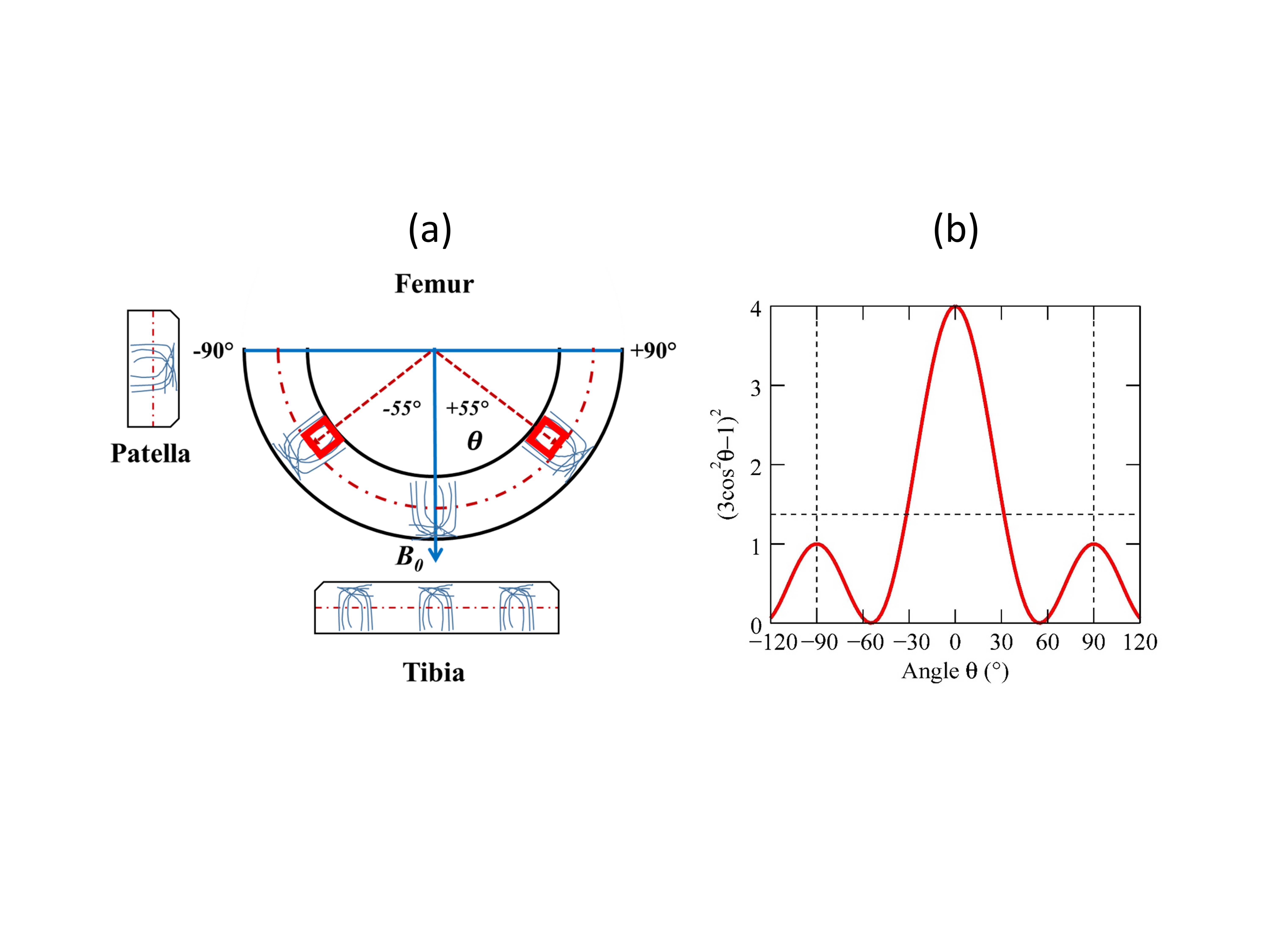
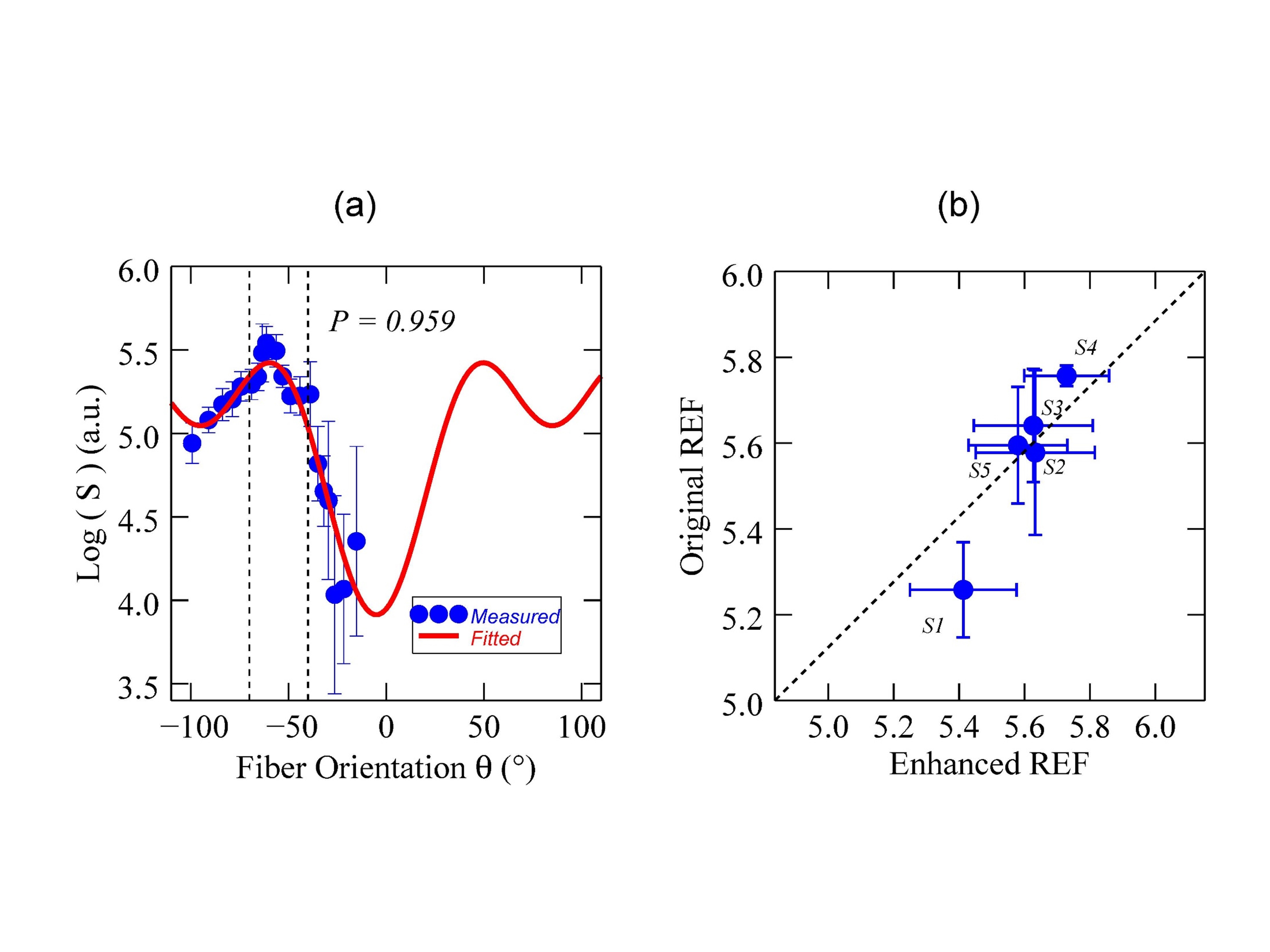
$$$R_2$$$ in cartilage at 3T can be considered as a weighted average of an isotropic $$${R_2^i}$$$ and an anisotropic $$${R_2^a (θ)}$$$³, leading to T2W signals $$$S(θ, TE)=S_0*exp({-TE*({R_2^i}+{R_2^a (θ)})},$$$ with $$${R_2^a (θ)}=R_2^a((1-3cos^2θ)/2)^2$$$. In deep cartilage, $$${R_2^a (θ)}$$$ vanishes when collagen fibers, predominantly perpendicular to the cartilage surface, are at magic angles $$$(θ=±55^o)$$$ to the main magnetic field $$$B_0$$$.^3,4 Given a constant “free” water contribution (as an internal reference, IR), $$${R_2^a (θ)}$$$ can be calculated as $$$(1/TE)log[S(θ=±55^o,TE)/S(θ,TE)]$$$, with TE of echo-time. IR can be derived from either a fit (“Original REF”) of $$$logS(θ,TE)$$$ to $$$a+b*(1-3cos^2θ)^2$$$ or a ranking method (“Enhanced REF”) of identifying local maxima near magic angle locations.

Four volunteers were enrolled and five knees $$$(S1-S5)$$$ were studied with $$$R_2$$$ and $$$R_{1ρ}$$$ mappings in sagittal plane on a Philips 3T MR scanner. T2W images were acquired using an interleaved MSME TSE pulse sequence, with an effective TE of n*6.1 ms (n=1,2,3,4,5,6,7,8) and a TR of 2500 ms. The acquired voxel size was 0.6*0.6*3.0 mm³ and the total scan time was 9 minutes. Five $$$R_{1ρ}$$$-weighed 3D images with different TSL (0, 10, 20, 30 and 40 ms) were acquired with a spin-lock (500 Hz) prepared T1-enhanced 3D TFE pulse sequence. The acquired voxel size was 0.40*0.40*3.00 mm³ and the total scan duration was 11 minutes.

After image co-registrations, $$$R_2$$$ and $$$R_{1ρ}$$$ pixel maps were created by curve-fittings based on a 2-parameter exponential decay model. $$${R_2^a (θ)}$$$ was derived from the ARCADE method in one T2W dataset (TE=48.8 ms) from $$$R_2$$$ mapping. An angular-radial segmentation was performed on femoral cartilage and each angularly segmented ROI was further subdivided equally into the deep and superficial zones.⁵ All image and data analysis was performed with an in-house software developed in IDL 8.5 (Exelis Visual Information Solutions, Boulder, CO).

RESULTS AND DISCUSSION

Fig. 1a shows schematically collagen fibers in three different cartilages and segmented femoral ROIs in deep zone at magic angles. The orientation dependence of normalized $$${R_2^a(θ)}$$$ is plotted in Fig. 1b, showing a value of 1.37 (a dashed horizontal line) when averaged between ±90°.

An example of an IR determination by two methods is demonstrated in Fig. 2a and the average IRs from all slices are compared in Fig 2b for five subjects. Similar IR values were obtained, but the “Enhanced REF” approach should be more robust when pathologies such as osteoarthritis occur at areas other than magic angle locations.

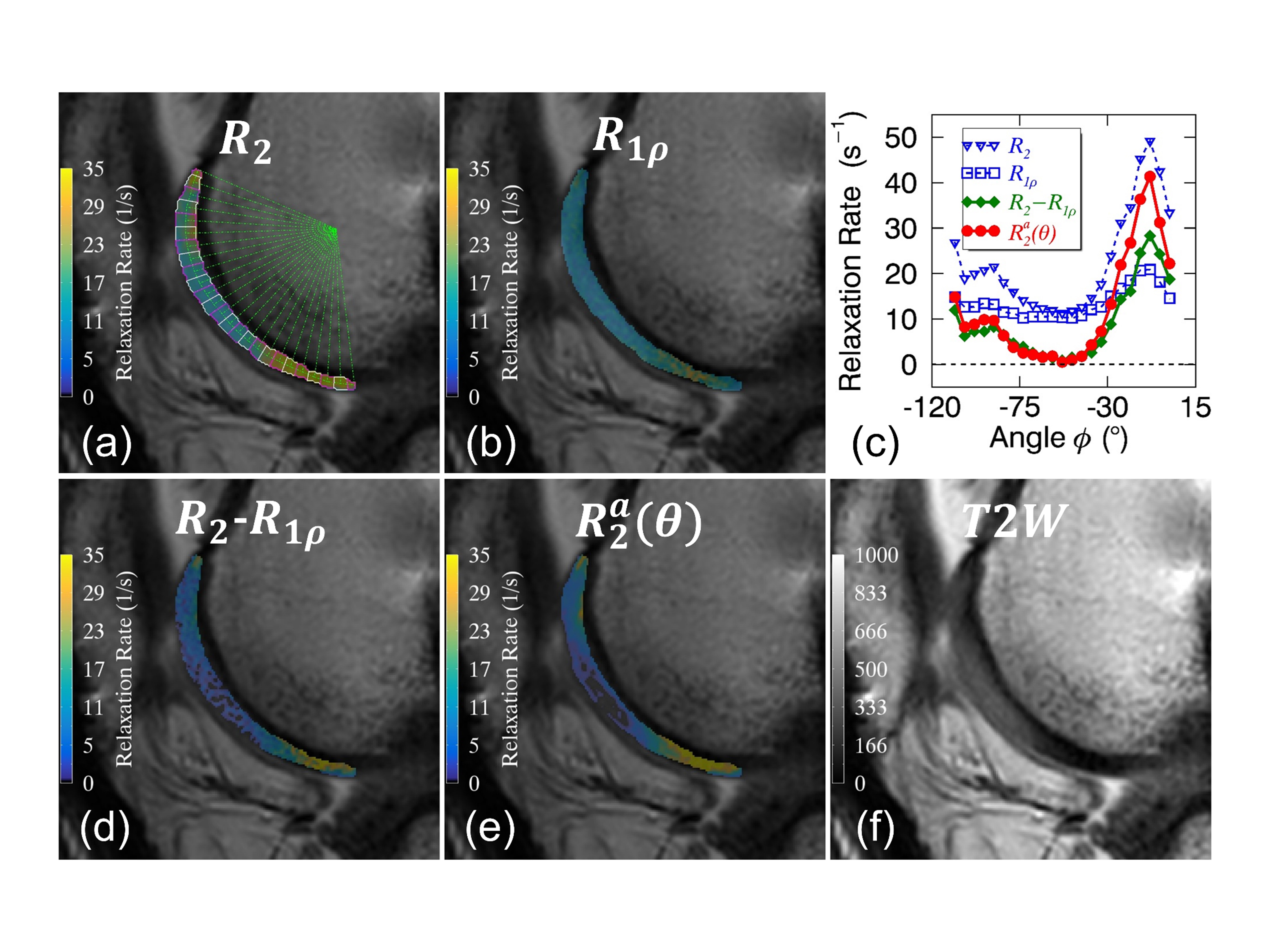
Fig. 3 presents parametric pixel maps of $$$R_2$$$(3a), $$$R_{1ρ}$$$(3b), $$$R_2-R_{1ρ}$$$(3d) and $$${R_2^a (θ)}$$$(3e) as well as a corresponding T2W (TE=48.8ms) anatomical image(3f) from subject S4. Clearly, $$$R_{1ρ}$$$(blue square) was reduced and less orientation-dependent compared with $$$R_2$$$(blue triangle) as reported,^1,6 and $$${R_2^a (θ)}$$$ (red circle) was hardly distinguishable from $$$R_2-R_{1ρ}$$$(green diamond) as shown in 3c.

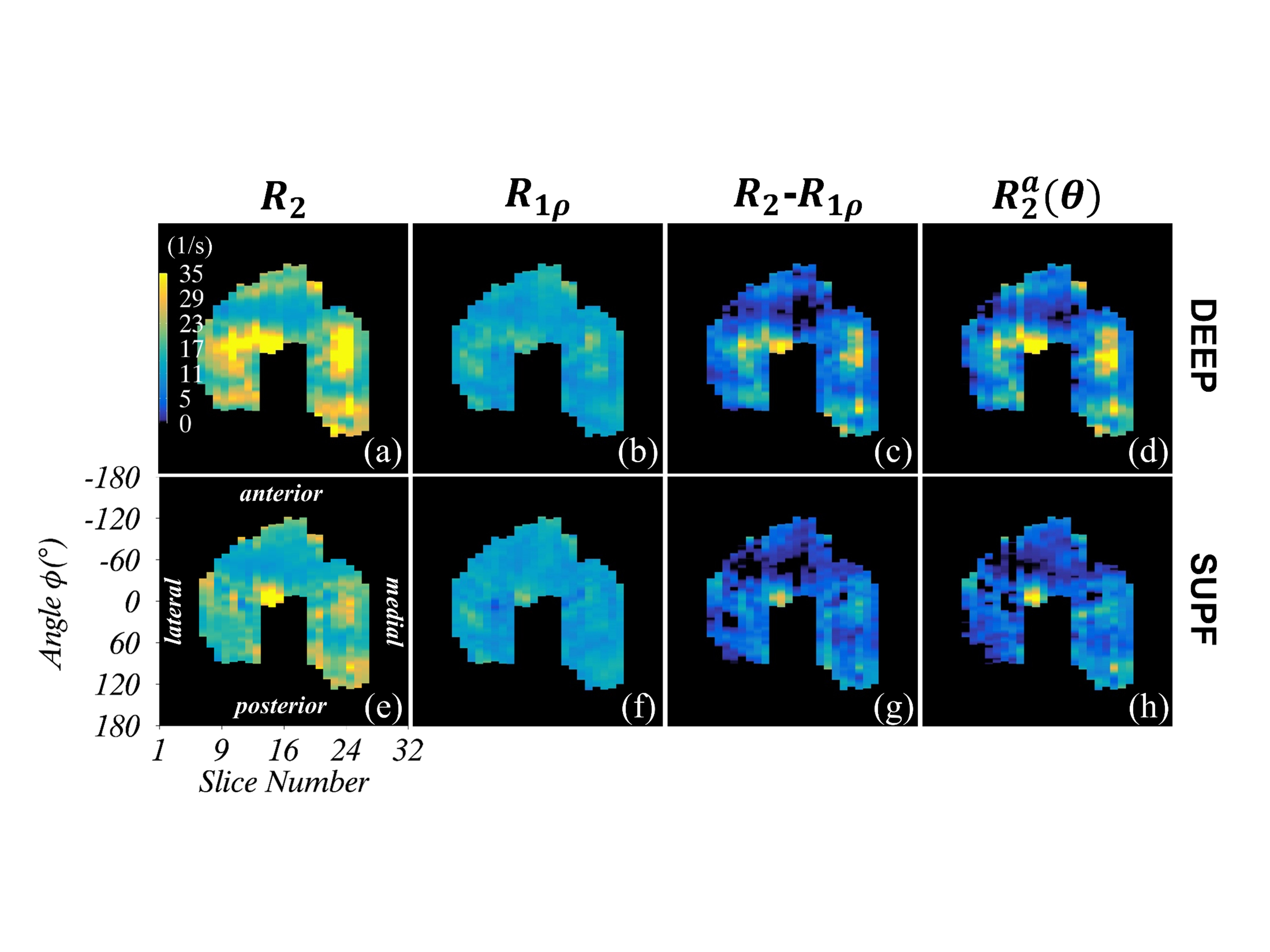
Derived from segmented femoral cartilage ROIs, parametric maps of $$$R_2$$$(4a,e), $$$R_{1ρ}$$$ (4b,f), $$$R_2-R_{1ρ}$$$(4c,g) and $$${R_2^a (θ)}$$$(4d,h) for all image slices of S4 are shown in Fig. 4 for the deep (4a-d) and the superficial (4e-h) zones. Generally, the trends observed in Fig. 3 were applicable to the whole cartilage, and all relaxation metrics had relatively higher values in the deep zone in agreement with previous findings.^1,4

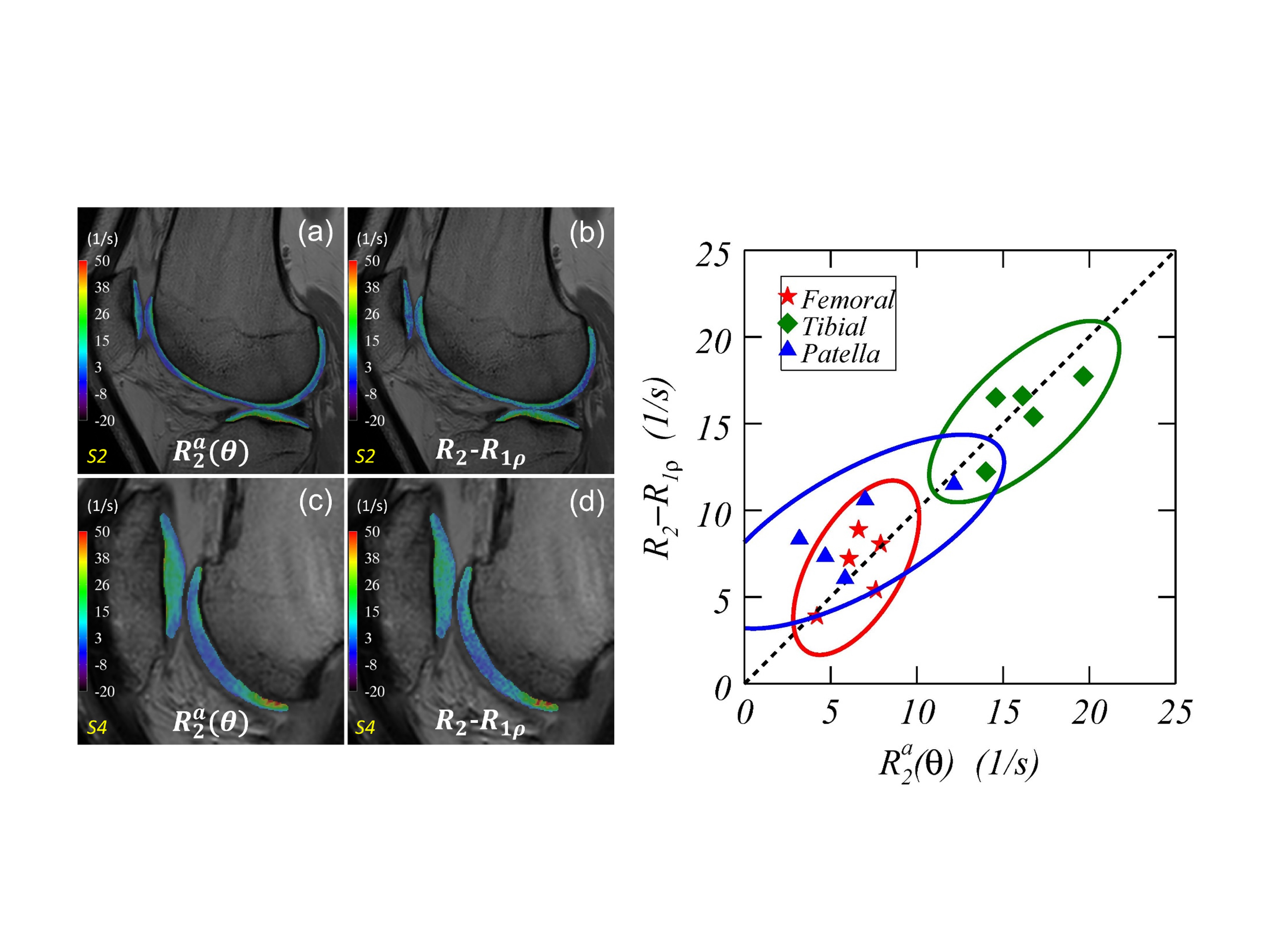
Besides femoral cartilage, $$${R_2^a (θ)}$$$(5a,c) was also qualitatively comparable to $$$R_2-R_{1ρ}$$$(5b,d) in the tibial and patella cartilages as demonstrated in Fig. 5a-d for subject S2 (5a-b) and subject S4 (5c-d). The average $$${R_2^a (θ)}$$$ within different cartilages for each of five knees was compared with that of $$$R_2-R_{1ρ}$$$ in a scatter-plot. The grand average of $$${R_2^a (θ)}$$$ (1/s) from five subjects was mostly comparable to that of $$$R_2-R_{1ρ}$$$ (1/s) in the femoral (6.5±1.5 vs. 6.7±1.5), tibial (16.3±2.2 vs.15.9±2.2) and patella (6.6±3.4 vs. 8.8±2.2) cartilages, indicating that an IR derived from the femoral cartilage was applicable to other knee cartilages as well. Moreover, the observed differences among three cartilages agreed well with theoretical predictions as shown in Fig. 1b, which could have been masked if an isotropic $$$R_2^i$$$ contribution had been included as reported in literature.

CONCLUSION

Acknowledgements

References

1. Hanninen N, Rautiainen J, Rieppo L, et al. Orientation anisotropy of quantitative MRI relaxation parameters in ordered tissue. Sci Rep 2017;7(1):9606.
2. Pang Y, Palmieri-Smith RM, Chenevert TL. A composite metric R2-R1ρ measures an incomplete anisotropic R2 of human femoral cartilage at 3T. In: Proceedings of the 26th Annual Meeting of ISMRM, Paris, France, 2018. (abstract 3104).
3. Momot KI, Pope JM, Wellard RM. Anisotropy of spin relaxation of water protons in cartilage and tendon. NMR Biomed 2010;23(3):313-324.
4. Xia Y. Magic-angle effect in magnetic resonance imaging of articular cartilage: a review. Invest Radiol 2000;35(10):602-621.
5. Kaneko Y, Nozaki T, Yu H, et al. Normal T2 map profile of the entire femoral cartilage using an angle/layer-dependent approach. J Magn Reson Imaging 2015;42(6):1507-1516.
6. Shao H, Pauli C, Li S, et al. Magic angle effect plays a major role in both T1rho and T2 relaxation in articular cartilage. Osteoarthritis Cartilage 2017;25(12):2022-2030.