1300
3D visualization of the cranial bone using fully automated segmentation based on ultra-short echo-time (UTE) imaging1Medical Physics Group, Institute of Diagnostic and Interventional Radiology, Jena University Hospital - Friedrich Schiller University Jena, Jena, Germany, 2Michael Stifel Center for Data-driven and Simulation Science Jena, Friedrich Schiller University Jena, Jena, Germany, 3Abbe School of Photonics, Friedrich Schiller University Jena, Jena, Germany, 4Center of Medical Optics and Photonics, Friedrich Schiller University Jena, Jena, Germany
Synopsis
To enable 3D-visualization of the cranial bone based on multi-echo ultra-short echo-time (UTE) data, a fully automated segmentation algorithm is presented. The algorithm concatenates several easy to implement processing steps while taking T2* maps calculated from three or more echoes or difference images calculated from the first two echoes of a UTE sequence as input. Comparison between a CT-based segmentation and the UTE-based segmentation showed very good agreement. The 3D visualization allowed easy assessment of the location and the course of cranial sutures as well as of diploic veins.
Introduction
By using ultra-short echo-time (UTE) imaging it is possible to directly image compact bone despite its very short T2* relaxation time1,2. Segmenting the cranial bone from the surrounding tissues, such as the skin and brain, is beneficial as regards its visualization and analysis. In this work, we describe a fully automated algorithm for segmenting the cranial bone based on multi-echo UTE data. The algorithm works by using either absolute difference images between UTE echoes or calculated T2* relaxation time maps. The segmented data can then be used to create 3D volumetric maps of the distribution of the T2* relaxation time over the cranial bone.Methods
For image acquisition, a 3D-multi-echo UTE sequence was used with isotropic resolution and short, hard pulse excitation1. Echo times were 0.12ms, 2.48ms and 4.84ms. Other parameters: 256x256x213 acquisition matrix, (200x200x167mm)³ FoV, 930Hz/px bandwidth, 35° flip angle, 7.5ms TR, 57min TA, two averages, 181136 readouts per k-space and fat saturation. Measurements were performed with two male volunteers (25 and 33 year old) without known pathologies on a 3T PRISMA scanner (Siemens Healthineers) using a vendor supplied 20-channel head coil. The second volunteer had recently undergone a transverse CT-head scan not related to the study and provided the imaging data for comparison. CT imaging resolution was 0.5x0.5x3.0mm³ acquired with a Siemens Emotion Duo. Image reconstruction and data analysis of the UTE data were performed offline using MATLAB. T2*-maps were calculated by squared mono-exponential fitting.
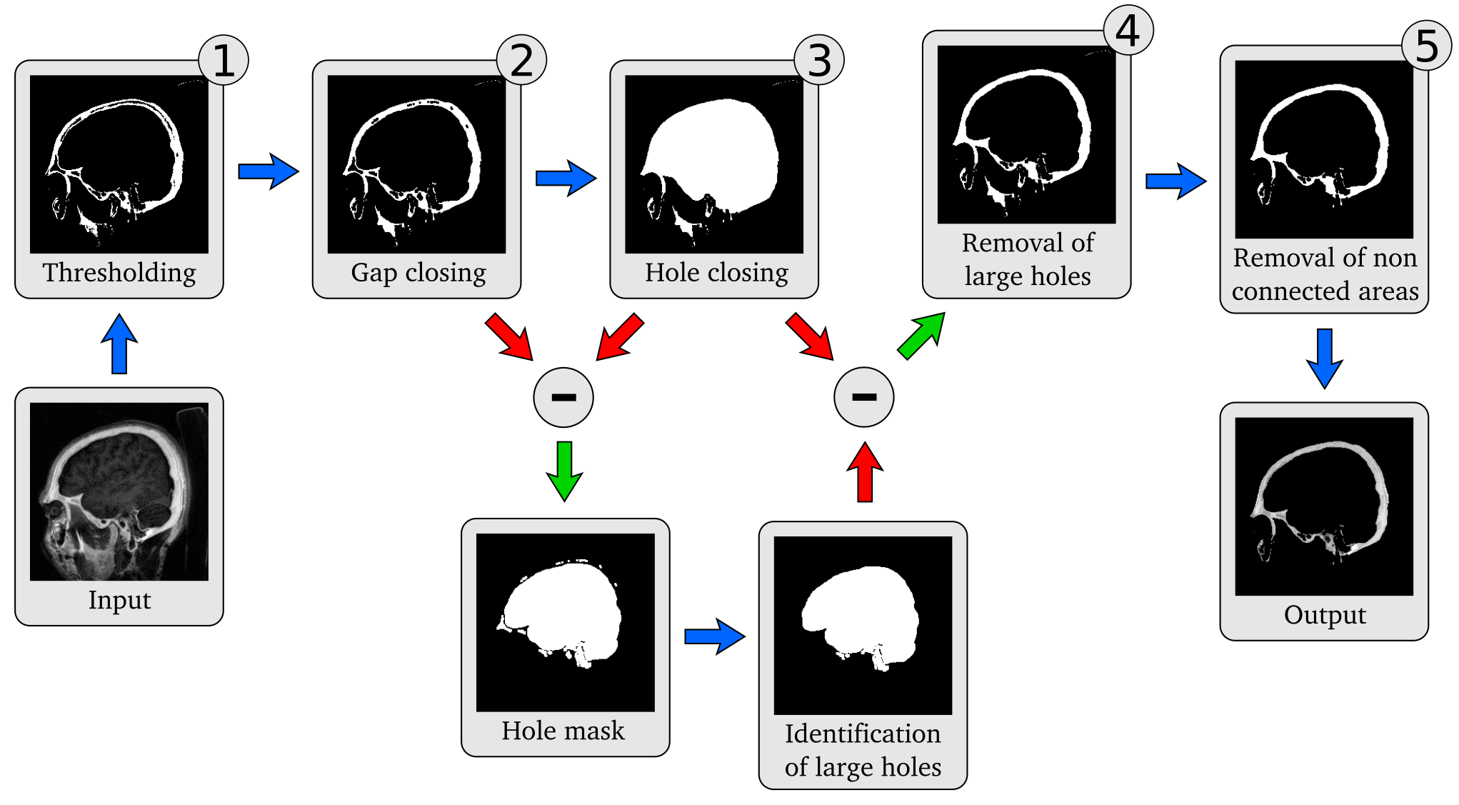
For automated segmentation of the cranial bone the following steps are performed:
- Thresholding: To create a binary base mask a threshold is applied. As input data either the absolute difference image between the magnitude images of the first and second echo or the calculated T2*-map is used. A threshold of 3 ms is applied to the T2*-map. When using the difference images for thresholding, a bias field correction3 is applied to homogenize signal intensities.
- Closing of gaps: Gaps in the outer contour of the cranial bone are removed by morphological closing, i.e., dilation following by erosion.
- Filling of holes: Remaining holes are closed by a flood-fill operation, which defines holes as all those regions that cannot be reached by filling in the background from the edges.
- Removal of large holes: Larger holes, such as the frontal sinus or an accidentally filled brain, are removed. Large holes are identified by finding connected components with a large number of pixels when considering the difference between (3) and (4).
- Removal of non-connected areas: Residual signal originating from cushions and pads, non-skull areas as well as other, non-connected areas is removed by analyzing the connectivity of all regions and retaining only the biggest connected object in the entire mask.
This optimized binary mask is then multiplied by the input data to segment the cranial bone. The segmentation algorithm is schematically depicted in Figure 1. Steps (2) and (3) are performed on a slice-by-slice basis in sagittal orientation. The other steps are applied on the entire 3D. 3D-visualization of the segmented cranial bone was performed by creating a semi-transparent volumetric rendering, where the respective T2*-values of each voxel were used for color encoding.
Results
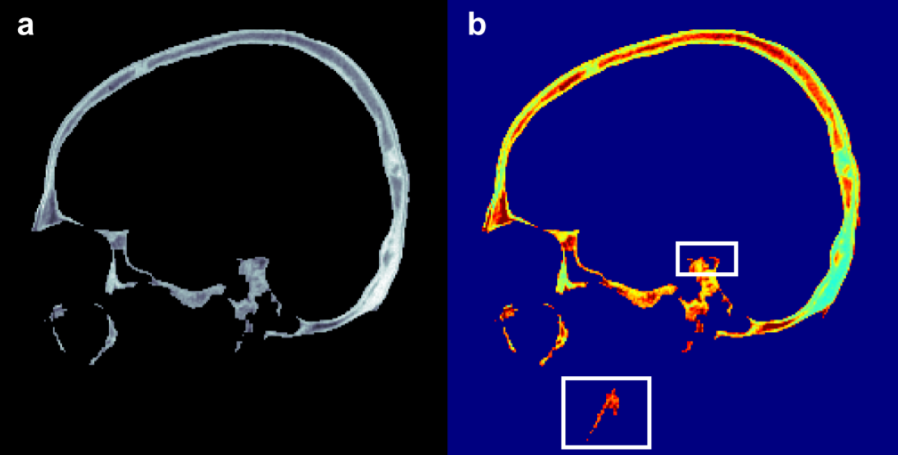
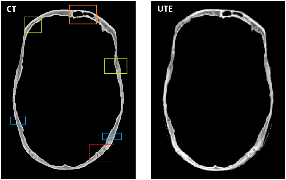
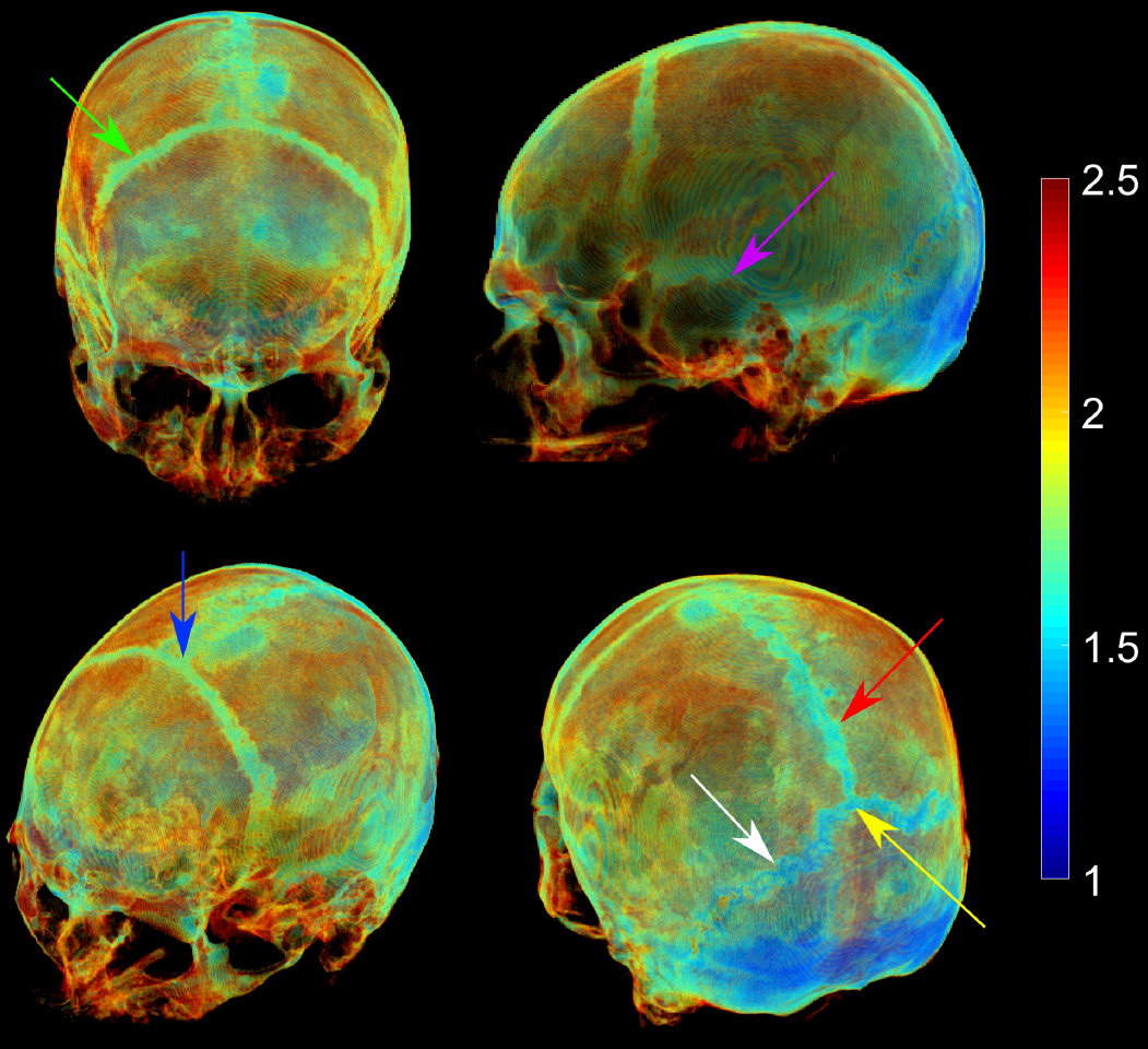
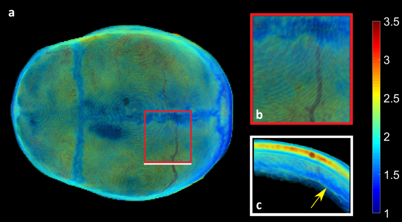
Figure 2 shows a segmented cranial bone for the two different inputs used. As seen, a clear segmentation was achieved in both cases with only few outliers. Comparing the MRI-based cranial bone segmentation to the transverse CT-scan (Fig. 3) revealed close agreement with only very few discrepancies. Details visible within the bone on the CT-scan were also visible on the UTE-based images. Volumetric 3D reconstruction of the segmented UTE data (Fig. 4) revealed a clear delineation of the cranial sutures due to their shortened T2*-times. A diploic vein was also visualized when viewing the calvaria from the top (Fig. 5).Discussion and Conclusion
Although T2*-map based segmentation showed a few more outliers after segmentation it was more robust since the threshold, which is applied as the first step for segmentation, can be chosen automatically based on known T2*-values of the cranial bone. Selecting a threshold for the difference images requires manual interaction, because the intensities depend on various factors, such as voxel size, receive coil, vendor or scanner-specific data sampling and processing. The presented segmentation algorithm consists of a concatenation of relatively simple and quick processing steps which are easy to implement. Comparison with CT-data revealed close agreement with the UTE segmentation, which is encouraging for potentially reducing CT-scans in some applications in the future. 3D volumetric renderings derived from the segmentation are advantageous in visualizing cranial bone which otherwise can only be partially viewed due to its bent and curved nature.Acknowledgements
Martin Krämer was supported by the German Research Foundation (DFG, RE 1123/22-1).References
- Herrmann KH, Krämer M, Reichenbach JR. Time Efficient 3D Radial UTE Sampling with Fully Automatic Delay Compensation on a Clinical 3T MR Scanner. PLoS One. 2016;Mar14;11(3):e0150371
- Robson MD, Gatehouse PD, Bydder M, Bydder GM. Magnetic resonance: An introduction to ultrashort TE (UTE) imaging. 2003. J Comput Assist Tomogr. 27(6):825–846.
- Tustison NJ, Avants BB, Cook PA, Zheng Y, Egan A, Yushkevich PA, and Gee JC. N4itk: Improved N3 bias correction. 2010. IEEE Trans Med Imaging, 29(6):1310–1320.
Figures