1249
Multi-Channel Image Reconstruction with Latent Coils and Adversarial Loss1Radiology, Stanford University, Stanford, CA, United States, 2Electrical Engineering, Stanford University, Stanford, CA, United States
Synopsis
Model-based accelerated imaging techniques enable high scan time reductions while maintaining high image quality. These techniques rely on the ability to accurately estimate the imaging model. This model can be extended to include information beyond physical limits, such as high-resolution phase information to promote conjugate symmetry or information of voxels without signal for a stronger image prior. Thus, we propose a deep learning approach to estimate the imaging model with latent coil maps. Furthermore, we jointly train this latent map estimator with a deep-learning-based reconstruction using adversarial loss, and we demonstrate the effectiveness of this approach in volumetric knee datasets.
Introduction
Model-based accelerated imaging techniques1–5 enable high scan time reduction (over 8 fold) while maintaining high image quality. At the core of these methods is the ability to accurately estimate the imaging model. This model characterizes the process of transforming the desired image to the measurement domain in k-space. A key component of the transform is the multi-channel coil array hardware. For optimal performance, coil profile maps must be characterized for each scan; however, the characterization can be costly in scan time and computation. Thus, we introduce a deep convolutional neural network (CNN) to estimate latent coil profile maps to model the imaging process. For further gains, this network is jointly trained with a reconstruction neural network with an adversarial loss.Method
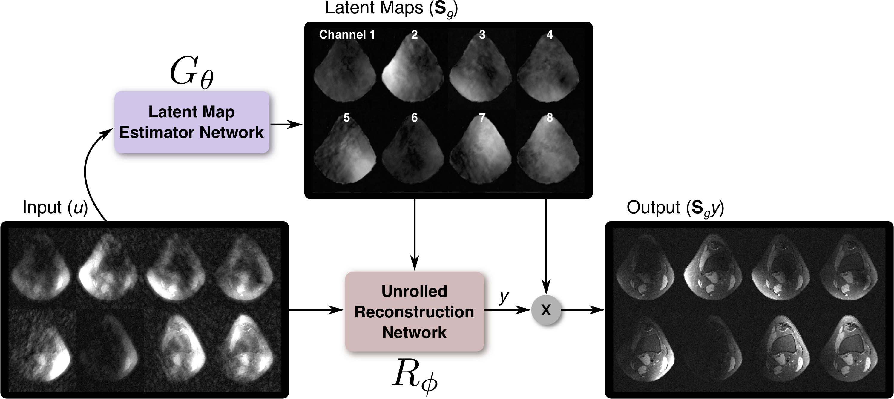
Current approaches to estimate the multi-channel model assume that each channel profile map of a coil array is slowly varying in space1–4. With accurate estimation (a) of voxels without signal and (b) of high spatial frequency components induced by field perturbations, additional information can be modeled by the profile map for improving the reconstruction. Thus, we propose to use unsupervised learning to avoid biasing our training based on previous methods: the CNN6 is trained based on how the output will be applied instead of on an ideal estimate of profile maps. More specifically, if the conjugate transpose of the maps estimated is applied to the original multi-channel, the number of channels is reduced (to 1 in this work). By applying the maps again, the result is the original multi-channel data. Because no constraint is imposed on the channel-reduced space and reconstruction will be performed in this space, we refer to the images in this space as latent coils and the profile maps as latent coil maps.
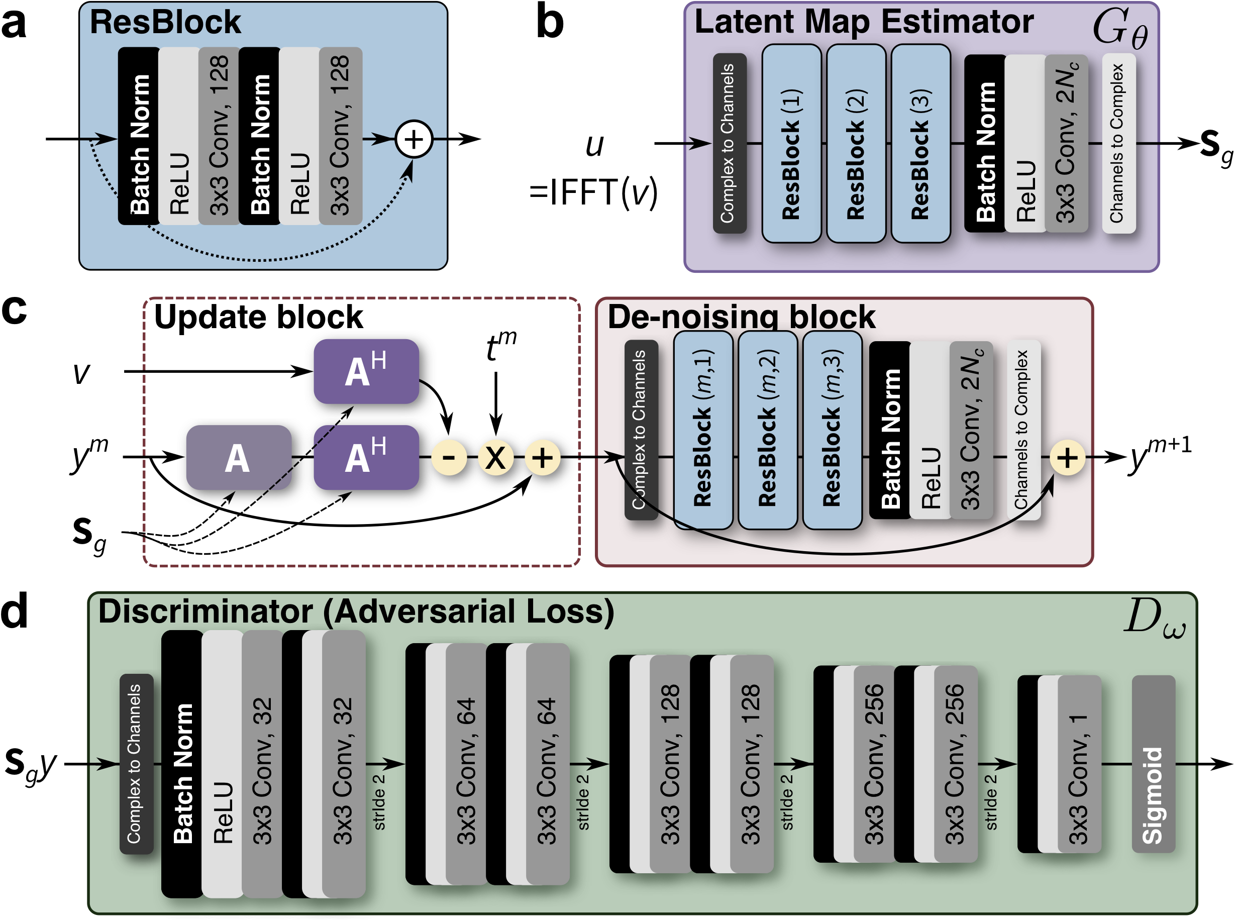
As the main goal is to improve the image reconstruction, the CNN for estimating these latent coil maps (Latent Map Estimator) are jointly trained with a reconstruction CNN based on compressed sensing7–9 (Reconstruction Network). Overview of the method is depicted in Figure 1. Furthermore, to improve the perceptual image quality of the reconstruction, adversarial loss (Discriminator, $$$D_\omega$$$) is used10.
The training consists of three components to the loss function. Latent map estimator $$$G_\theta$$$ (Figure 2b) is trained with loss: $$\mathcal{L}_L^\theta=\sum_i\left\|G_\theta(u_i)G^H_\theta(u_i)c_i-c_i \right\|_1,$$ where $$$c_i$$$ is the $$$i$$$-th fully-sampled multi-channel training example, and $$$u_i$$$ is k-space subsampled according to the subsampling mask used for future scans. Both $$$u_i$$$ and $$$c_i$$$ are in the image domain. $$$G_\theta$$$ is jointly trained with the reconstruction network $$$R_\phi$$$ (Figure 2c) with an additional loss: $$\mathcal{L}_R^{\theta,\phi}=\sum_i \left\|G_\theta(u_i)R_\phi(u_i,G_\theta(u_i))-c_i \right\|_1-\lambda\log(D_\omega(G_\theta(u_i)R_\phi(u_i,G_\theta(u_i)))),$$ where $$$R_\phi(u_i,G_\theta(u_i))$$$ outputs a latent image which is then transformed into the multi-channel image domain with $$$G_\theta(u_i)$$$. Discriminator $$$D_\omega$$$ (Figure 2d) is trained with loss $$$\mathcal{L}_D^{\omega}$$$: $$\mathcal{L}_D^{\omega}=\sum_i-\log(D_\omega(c_i))-\log(1-D_\omega(R_\phi(u_i,G_\theta(u_i)))),$$ where $$$D_\omega$$$ classifies each image patch as the original fully-sampled $$$c_i$$$ or not.
Proton-density-weighted volumetric knee scans11,12 using an 8-channel knee coil were used. Cartesian k-space data were first transformed into the hybrid $$$(x,ky,kz)$$$-space and separated into $$$x$$$-slices. Dataset consisted of 14, 2, and 3 knee subjects (4480, 640, and 960 slices) for training, validation, and testing. For training and for final testing, variable-density poisson-disc sampling masks were used. The networks were jointly trained in TensorFlow13; comparisons were performed using BART14.
Results
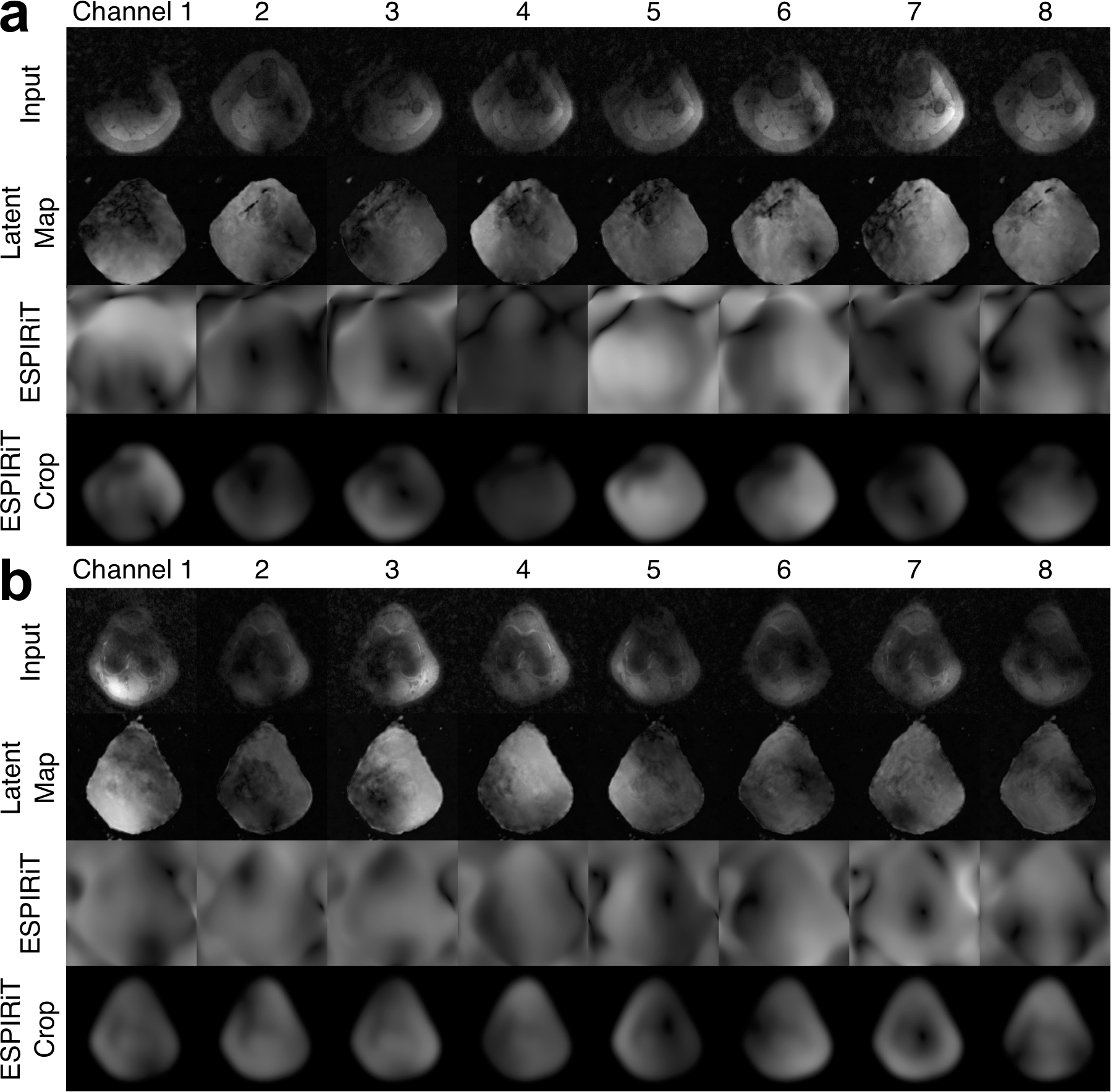
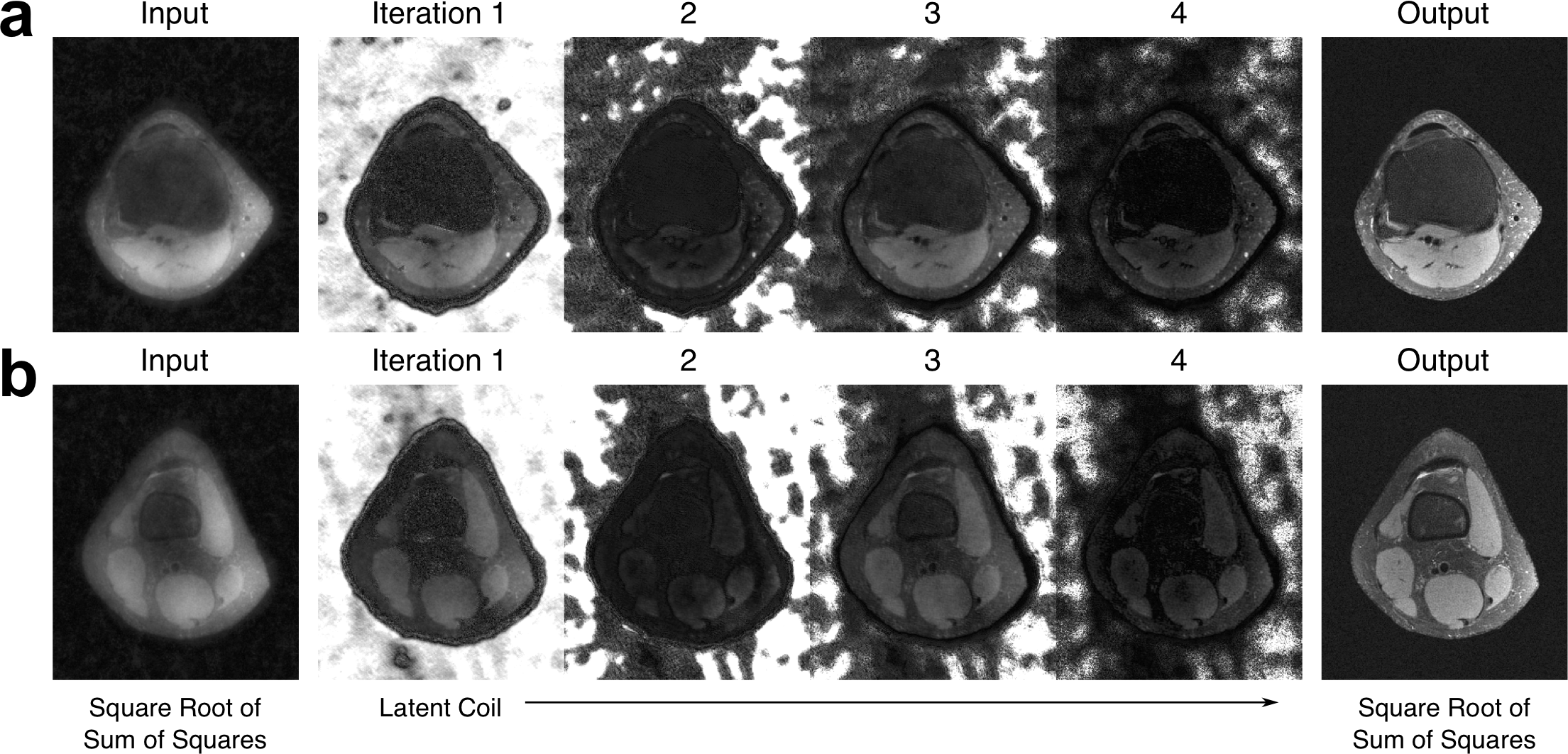
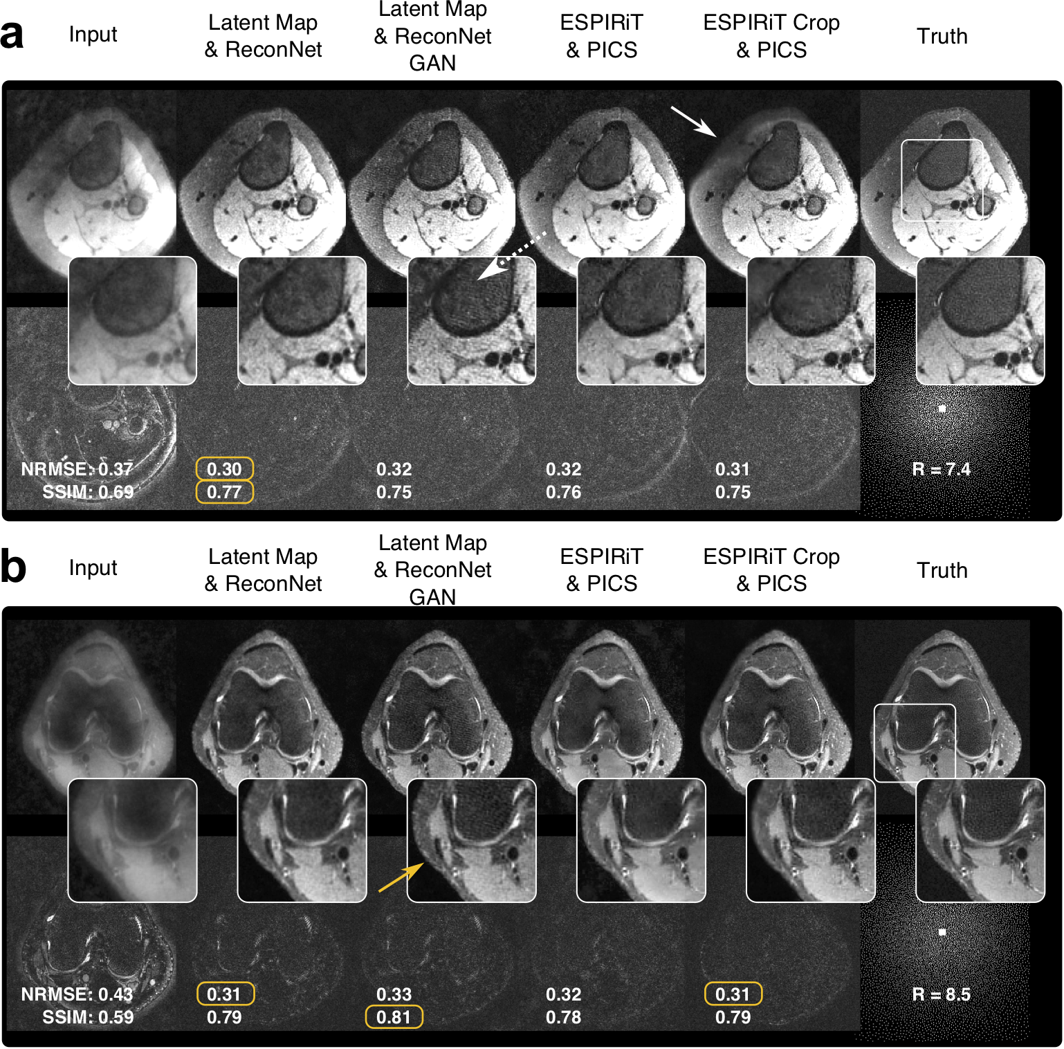
From a subsampled image set, latent coil maps were generated with high spatial frequencies (Figure 3). These latent coil maps were similar to the maps computed from ESPIRiT with and without automatic cropping. These latent coil maps were used to assist in the reconstruction of the subsampled dataset by transforming the multi-channel image into a latent space that is specific for de-noising (Figure 4). Reconstruction results for different approaches are shown in Figure 5. On a NVIDIA 1080 Ti card, the latent coil map CNN took 40ms and reconstruction CNN took 60ms, whereas ESPIRiT took 600ms and 9.6s without and with cropping. On the same GPU, parallel imaging & compressed sensing (PICS) with 30 iterations took 2.6s. The reconstruction network trained without adversarial loss appears smoother agreeing with previous literature10,15 whereas the network trained with adversarial loss has more high-resolution texture.Discussion & Conclusion
A single latent coil is used in this work, but the network can be easily extended to support more coils. The latent space enabled by the unsupervised training provides an unexplored domain for reconstruction solutions. Further, the proposed highly-flexible method allows for arbitrary regularizations to guide the unsupervised training and for training with arbitrary reconstruction networks. In conclusion, a CNN framework is proposed and trained with unsupervised learning to estimate latent coil maps. Latent coil maps are rapidly estimated and used for reconstructing multi-channel images.Acknowledgements
NIH R01-EB009690, NIH R01-EB019241, NIH R01-EB026136, and GE Healthcare.References
- Griswold, M. A. et al. Generalized autocalibrating partially parallel acquisitions (GRAPPA). Magn. Reson. Med. 47, 1202–1210 (2002).
- Pruessmann, K. P., Weiger, M., Scheidegger, M. B. & Boesiger, P. SENSE: sensitivity encoding for fast MRI. Magn. Reson. Med. 42, 952–62 (1999).
- Lustig, M. & Pauly, J. M. SPIRiT: Iterative self-consistent parallel imaging reconstruction from arbitrary k-space. Magn. Reson. Med. 64, 457–471 (2010).
- Uecker, M. et al. ESPIRiT-an eigenvalue approach to autocalibrating parallel MRI: Where SENSE meets GRAPPA. Magn. Reson. Med. 71, 990–1001 (2014).
- Lustig, M., Donoho, D. & Pauly, J. M. Sparse MRI: The application of compressed sensing for rapid MR imaging. Magn. Reson. Med. 58, 1182–1195 (2007).
- He, K., Zhang, X., Ren, S. & Sun, J. Identity Mappings in Deep Residual Networks. arXiv:1603.05027 [cs.CV] (2016).
- Hammernik, K. et al. Learning a variational network for reconstruction of accelerated MRI data. Magn. Reson. Med. 79, 3055–3071. PMCID: PMC5902683 (2018).
- Diamond, S., Sitzmann, V., Heide, F. & Wetzstein, G. Unrolled Optimization with Deep Priors. arXiv: 1705.08041 [cs.CV] (2017).
- Cheng, J. Y., Chen, F., Alley, M. T., Pauly, J. M. & Vasanawala, S. S. Highly Scalable Image Reconstruction using Deep Neural Networks with Bandpass Filtering. arXiv:1805.03300 [cs.CV] (2018).
- Mardani, M. et al. Deep Generative Adversarial Neural Networks for Compressive Sensing (GANCS) MRI. IEEE Trans. Med. Imaging (2018). doi:10.1109/TMI.2018.2858752
- Epperson, K. et al. Creation of Fully Sampled MR Data Repository for Compressed Sensing of the Knee. in SMRT 22nd Annual Meeting (2013). doi:10.1.1.402.206
- MRI Data. Available at: http://mridata.org/. (Accessed: 14th July 2017)
- Abadi, M. et al. TensorFlow: Large-Scale Machine Learning on Heterogeneous Distributed Systems. arXiv:1603.04467 [cs.DC] (2016).
- Uecker, M. et al. BART: version 0.3.01. (2016). doi:10.5281/zenodo.50726
- Pathak, D., Krahenbuhl, P., Donahue, J., Darrell, T. & Efros, A. A. Context Encoders: Feature Learning by Inpainting. in 2016 IEEE Conference on Computer Vision and Pattern Recognition (CVPR) 2536–2544 (IEEE, 2016). doi:10.1109/CVPR.2016.278
Figures