1122
Towards QSM Challenge 2.0: Creation and Evaluation of a Realistic Magnetic Susceptibility Phantom1Donders Institute for Brain Cognition and Behaviour, Radboud University, Nijmegen, Netherlands, 2Athinoula A. Martinos Centre for Biomedical Imaging, Charlestown, MA, United States, 3Department of Radiology, Harvard Medical School, Boston, MA, United States, 4Harvard-MIT Health Sciences and Technology, MIT, Cambridge, MA, United States, 5Philips Research, Hamburg, Germany, 6Department of Electrical Engineering, Pontificia Universidad Catolica de Chile, Santiago, Chile, 7Biomedical Imaging Center, Pontificia Universidad Catolica de Chile, Santiago, Chile, 8Spinoza Centre for Neuroimaging, Amsterdam, Netherlands, 9Department of Neurology, Medical University of Graz, Graz, Austria, 10Buffalo Neuroimaging Analysis Center, Department of Neurology, Jacobs School of Medicine and Biomedical Sciences, University at Buffalo, The State University of New York, Buffalo, NY, United States, 11Center for Biomedical Imaging, Clinical and Translational Science Institute, University at Buffalo, The State University of New York, Buffalo, NY, United States
Synopsis
We present the creation of a modular and realistic digital phantom to serve as a ground-truth to assess the quality of different reconstruction algorithms for Quantitative Susceptibility Mapping (QSM). The phantom is derived from high-resolution, quantitative MRI data of a healthy volunteer, features a realistic morphology including a non piece-wise constant susceptibility distribution. Varying degrees of complexity can be realized, for example by adding the effects of tissue microstructure, down sampling or adding background-fields. The freely available phantom will be used in the upcoming QSM Reconstruction challenge.
Motivation
Quantitative Susceptibility Mapping (QSM) is today an established method to study iron accumulation in the deep gray matter (DGM) and demyelinating lesions in the white matter (WM). However, despite its usefulness for studying disease pathogenesis, several recent studies have suggested that study outcomes may be affected by the particular phase processing algorithms chosen for QSM.1–3
The 2016 QSM Reconstruction Challenge (RC) aimed to provide insights on the ability of QSM algorithms to reconstruct in vivo brain susceptibility accurately.4 The outcome of the challenge was partly inconclusive because the employed ground truth (GT) was obtained via susceptibility tensor imaging (STI),5 which appropriately disentangles phase effects related to susceptibility anisotropy that are not disentangled by current single-orientation QSM techniques. As a result, most RC submissions with low error metrics were over-smoothed or piecewise constant due to over-regularization.
Here, the design of a customized realistic digital brain phantom generated from quantitative parameter maps of one volunteer is presented. Its performance as a GT for the upcoming RC is evaluated and the design of the 2019 QSM Reconstruction Challenge is announced.
Design of the Realistic Brain Phantom:
The phantom is based on data from a human volunteer (F, 38 years). High resolution (0.64mm isotropic) quantitative maps of R1 7, R2*, $$$\chi$$$8, and M0 were obtained with the MP2RAGEME6 sequence at 7T (Philips; TR/TI1/TI2=6.72/0.67/3.86s TE1-4=3/11.5/20/28.5ms, α1/α2 = 7/6 o). High resolution T1w (0.8mm) data at zero echo time was acquired using the PETRA9 sequence and two DWI (1.5mm) datasets with b=~0/1250/2500s/mm² and 12/90/90 directions at 3T (Siemens PrismaFIT).
Once the most relevant structures (CSF, GM, WM, veins, various DGM nuclei, bone and air) were segmented using the pipeline described in Figure 1, we created a susceptibility map with each segmented tissue being attributed literature susceptibility values 10,11. To avoid piece-wise constant regions, susceptibility values in each region were modulated using R1 and R2* maps so that:
$$ \chi(r) = \overline{ \chi_{tissue}} + a_{tissue} (R_2^{*}(r)-\overline{R^{*}_{2tissue}}) + b_{tissue} (R_1(r)-\overline{R_{1tissue}}) [Eq 1] $$
To smooth the transition between segmented tissues, the probability of being a given tissue, Ptissue, was computed by smoothing each tissue binary mask by a Gaussian of FWHM 1.2 voxels. The susceptibility model was then:
$$ \chi(r) = \sum_{tissue=1}^{15} P_{tissue}(r)\chi_{tissue}(r) [Eq2]$$
We simulated a multi-echo acquisition (TR/TEs=50/4/12/20/28, see Fig.3). As a GT and for background field correction purposes, we eliminated the effect of magnetic susceptibilities outside the brain (and a calcification inside the brain) and demeaned the susceptibility values elsewhere. A lower resolution version of the complex data (1mm isotropic) was computed by k-space cropping. Low-resolution GT susceptibility maps were created via interpolation to avoid oscillatory errors associated with k-space cropping.
Evaluation of Phantom on a Reconstruction Challenge scenario:
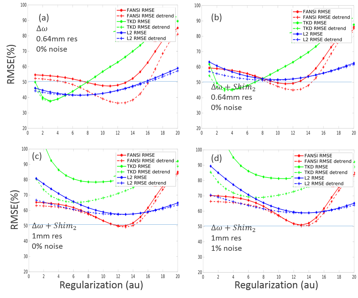
Complex data free of skull, muscle tissue and air susceptibility perturbations was simulated at two different SNR levels (Infinite SNR and 100) and resolutions (0.64 and 1mm). Fieldmaps were computed by complex model fitting and subsequently processed by three QSM12–14 algorithms: k-space threshold (TKD), single-step l2 regularization, and FANSI. The solutions found were compared to the GT using RMSE with and without compensation for systematic underestimation.
Figure 4
shows plots of the reconstruction errors as a function of regularization
factors for the 2016 RC and the proposed novel model. The optimum
reconstructions for different metrics were evaluated and the current metric provided
lower RMSE solutions that are not as (piece-wise) smooth as in the previous
challenge. The
large RMSE values observed (for a phantom) are a result of the
various nuisances introduced: such as the additional polynomial field (Fig.5b),
the down-sampling to 1mm (Fig.5c) procedure and noise (Fig.5d). All thes processes increase the optimum regularization found.
2019 QSM Reconstruction Challenge Design:
The goal of the RC-2019 is to provide insights on the current state of the art in QSM algorithms and identify their strengths and limitations in different scenarios. The challenge will consist of two stages: Stage I will mimic the clinical setting in which the ground-truth is unknown; in Stage 2 the ground truth will be available and thus allow systematic parameter optimizations for the best possible quality metrics that can be obtained with a specific reconstruction algorithm. Results will be presented at the 2019 QSM Workshop in Seoul, Korea. The code for the generation of the current model and synthetic data will be then made publicly available.Conclusion:
The presented realistic and modular phantom will serve as a GT for the QSM RC and generally enable researchers to optimize reconstruction as well as acquisition parameters. Its modular design allows adding microstructure effects a posteriori15 as well as the inclusion of new nuisances such as haemorrhages or fine vessels with realistic relaxation and susceptibility properties.Acknowledgements
The authors would like to acknowledge the fruitful discussions with Drs. Karin Shmueli, Julio Acosta-Cabronero, Pascal Spincemaille, Ludovic de Rochefort, Cristian Tejos, and Pinar Özbay.References
1. Robinson, S. D. et al. An illustrated comparison of processing methods for MR phase imaging and QSM: combining array coil signals and phase unwrapping. NMR Biomed. 30, e3601 (2017).
2. Wang, Y. & Liu, T. Quantitative susceptibility mapping (QSM): Decoding MRI data for a tissue magnetic biomarker. Magn. Reson. Med. 73, 82–101 (2015).
3. Schweser, F., Robinson, S. D., de Rochefort, L., Li, W. & Bredies, K. An illustrated comparison of processing methods for phase MRI and QSM: removal of background field contributions from sources outside the region of interest. NMR Biomed. n/a-n/a (2016). doi:10.1002/nbm.3604
4. Langkammer, C. et al. Quantitative susceptibility mapping: Report from the 2016 reconstruction challenge. Magn. Reson. Med. (2017). doi:10.1002/mrm.26830
5. Liu, C. Susceptibility tensor imaging. Magn. Reson. Med. 63, 1471–1477 (2010).
6. (ISMRM 2018) MP2RAGEME: T1, T2* and QSM mapping in one sequence at 7 Tesla. Available at: http://archive.ismrm.org/2018/0034.html. (Accessed: 6th November 2018)
7. Marques, J. P. et al. MP2RAGE, a self bias-field corrected sequence for improved segmentation and T1-mapping at high field. NeuroImage 49, 1271–1281 (2010).
8. Schweser, F., Sommer, K., Deistung, A. & Reichenbach, J. R. Quantitative susceptibility mapping for investigating subtle susceptibility variations in the human brain. NeuroImage 62, 2083–2100 (2012).
9. Grodzki, D. M., Jakob, P. M. & Heismann, B. Ultrashort echo time imaging using pointwise encoding time reduction with radial acquisition (PETRA). Magn. Reson. Med. 67, 510–518 (2012).
10. Deistung, A. et al. Toward in vivo histology: a comparison of quantitative susceptibility mapping (QSM) with magnitude-, phase-, and R2*-imaging at ultra-high magnetic field strength. NeuroImage 65, 299–314 (2013).
11. Buch, S. et al. Susceptibility mapping of air, bone, and calcium in the head. Magn. Reson. Med. 73, 2185–2194 (2015).
12. Shmueli, K. et al. Magnetic susceptibility mapping of brain tissue in vivo using MRI phase data. Magn. Reson. Med. Off. J. Soc. Magn. Reson. Med. Soc. Magn. Reson. Med. 62, 1510–1522 (2009).
13. Bilgic, B. et al. Fast image reconstruction with L2-regularization. J. Magn. Reson. Imaging n/a–n/a (2013). doi:10.1002/jmri.24365
14. Milovic, C., Bilgic, B., Zhao, B., Acosta‐Cabronero, J. & Tejos, C. Fast nonlinear susceptibility inversion with variational regularization. Magn. Reson. Med. 80, 814–821 (2018).
15. Wharton, S. & Bowtell, R. Effects of white matter microstructure on phase and susceptibility maps. Magn. Reson. Med. Off. J. Soc. Magn. Reson. Med. Soc. Magn. Reson. Med. (2014). doi:10.1002/mrm.25189
16. Manniesing, R., Viergever, M. A. & Niessen, W. J. Vessel enhancing diffusion: a scale space representation of vessel structures. Med. Image Anal. 10, 815–825 (2006).
Figures


Figure 2: Coronal and transverse slices (and zoomed insert at the region of the Globus Pallidus with a changed colorscale) of different susceptibility models: (a) Piece-wise constant; (b) Modulated using Eq.1 (c) Probability + Modulated using Eq. 1 and 2 (note that tissue interfaces become smoother, particularly close to veins, become smoother) (d) As in c, but with tissue modulation parameters further enhanced by a factor 2.

Additional considerations for mimicking real-world data. Realistic data was simulated using the GRE steady state equation:
$$$ S(r)=exp(-TE.R_2^* +i(\phi(r) +TE.(\Delta \omega_{\chi} - Shim_2)) ) SS(\alpha,TR,R_1(r)) $$$
Where (a) Φ(r) is a smoothly varying transceiver phase, (b) Δω represents the field computed using the standard dipole relationship and Shim2 represents a second order polynomial fitted to the brain region to increase homogeneity in the brain (c). The simulated data magnitude and phase data (d) with $$$TR/TE/\alpha=50ms/28ms/15^o$$$ corresponds nicely to the acquired data (f). If desired, microstructural effects (e) can be added at later stages using the DTI data.