1113

Intact Metabolite Spectrum Mining by Deep Learning in Proton Magnetic Resonance Spectroscopy of the Brain

HyeongHun Lee¹ and Hyeonjin Kim^1,2

¹Department of Biomedical Sciences, Seoul National University, Seoul, Korea, Republic of, ²Department of Radiology, Seoul National University Hospital, Seoul, Korea, Republic of

Synopsis

¹H-MRS can quantify brain metabolites noninvasively. However, in a typical clinical setting, human brain spectra are indispensably degraded due to low SNR, line-broadening, and unknown spectral baseline, and consequently, quantification of brain metabolites is challenging even with the current state-of-the-art software. Given the recent accomplishment of deep-learning in a variety of different tasks, we developed a convolutional-neural-network (CNN) that maps the degraded brain spectra into noise-free, line-narrowed, baseline-removed, metabolite-only spectra. The robust performance of the proposed method as validated on both simulated and in vivo human brain spectra strongly supports the potential of deep learning in ¹H-MRS of human brain.

Target Audience

Those interested in metabolite quantification in ¹H-MRS using deep learning.

Introduction

In a typical clinical setting, brain spectra are degraded due to low SNR, line-broadening, and spectral baseline. To quantify individual metabolites from the degraded brain spectra, a nonlinear least-squares fitting is the most widely used approach.^1,2 However, even with the current state-of-the-art software, it is challenging.³ Therefore, development of a robust method for brain metabolite quantification is a remaining issue in ¹H-MRS.

Given the recent accomplishment of deep learning in a variety of different tasks, ^4,5 we developed a convolutional-neural-network (CNN) that maps degraded in vivo brain spectra into noise-free, line-narrowed, baseline-removed, metabolite-only spectra. The subsequent metabolite quantification from the metabolite-only spectra is achieved by solving a simple inverse problem. The performance of the proposed method was tested on both simulated and in vivo human brain spectra.

Methods

In vivo data: The study was approved by IRB (5 healthy volunteers). In vivo spectra were collected from the left frontal lobe using PRESS at 3.0T (Siemens; TR/TE=2000/30ms, SW=2kHz, 2048 points, voxel size=8cm³, and 64 averages).

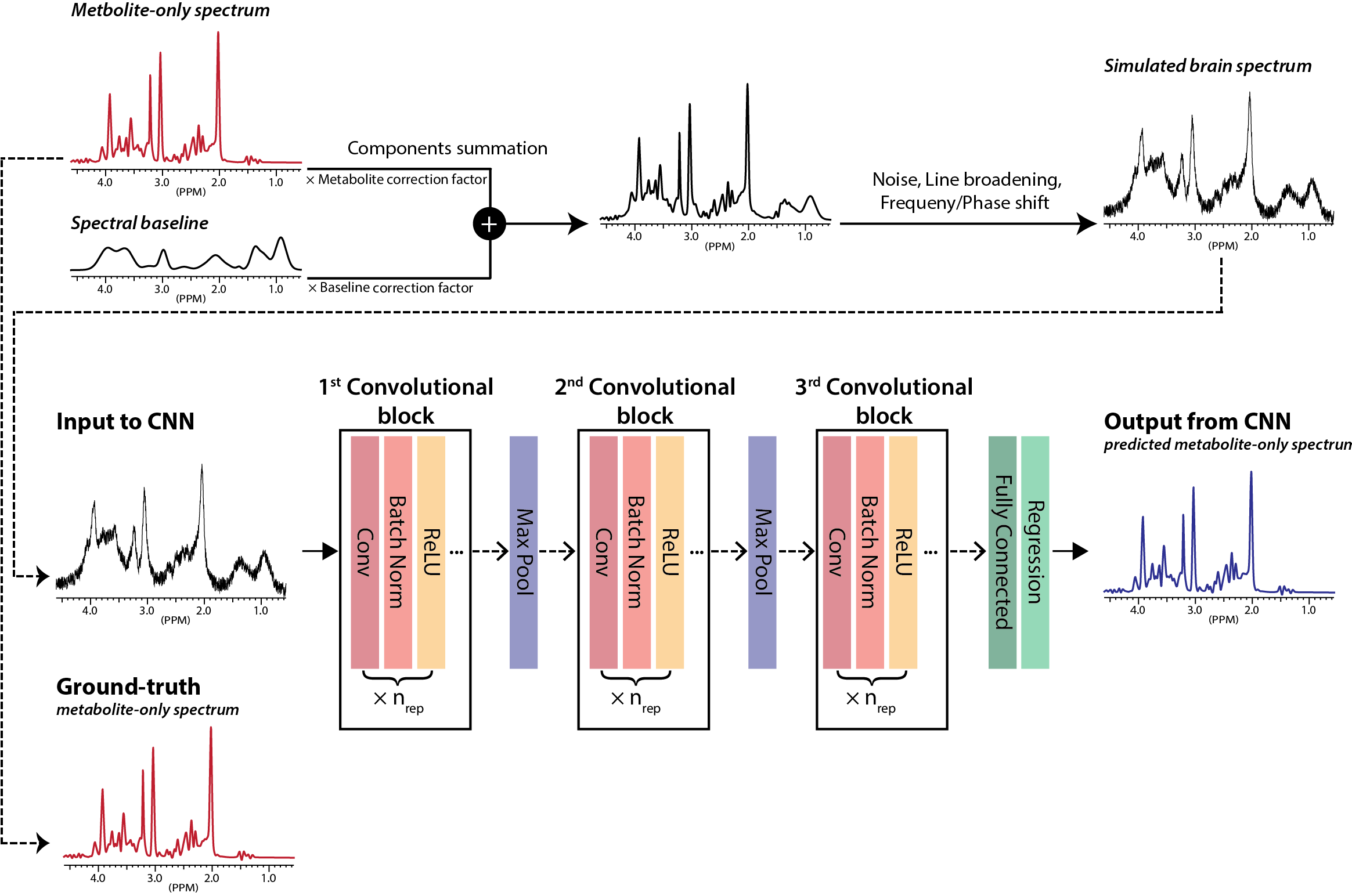
Brain spectra simulation: Based on the previous studies, ^6-9 the upper/lower bounds of the metabolite concentrations in normal human brain were defined for 17 metabolites. First, metabolite-only spectra were simulated by combining all individual metabolite phantom spectra according to randomly varying relative metabolite concentration ratios within the concentration bounds. These metabolite-only spectra were used as the ground-truth target spectra (Fig.1). Second, spectral baseline was simulated by using 17 Gaussian functions with randomly varying relative amplitudes within ±10% from the reported ranges.^10,11 Third, the metabolite-only spectra and the baseline spectra were combined by randomly varying their relative ratio within ±10% from a predetermined ratio.¹² Forth, line-broadening, noise, and frequency/phase shift were applied to the combined spectra. Finally, 50000 spectra were simulated and assigned to a training (N=40000), a validation (N=5000) and a test (N=5000) sets.

CNN: A CNN was designed and Bayesian-optimized ¹⁴ in Matlab (Mathworks Inc) (Fig.1).

Metabolite quantification: The quantification of individual metabolites from the CNN-predicted metabolite-only spectra was achieved by solving an inverse problem. That is, C = S pinv(b) (C: matrix containing the relative concentrations of the 17 metabolites, S: matrix containing the CNN-predicted spectra, pinv: pseudoinverse of a matrix, and b: matrix containing the basis spectra of the 17 metabolites).

Evaluation of the proposed method: Using the simulated spectra in the test set, the proposed method was evaluated by calculating the mean-absolute-percent-error (MAPE) between the ground-truth and the metabolite concentrations estimated by the proposed method. Using in vivo spectra, the quantification results from the proposed method were compared with those from the LCModel analysis.

Results

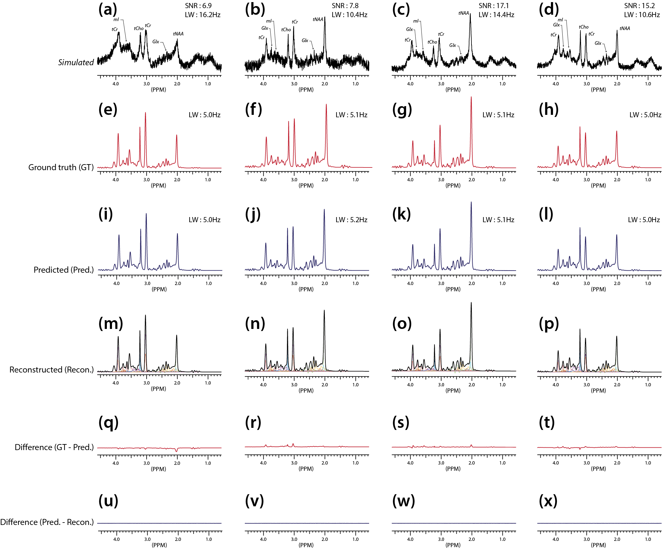
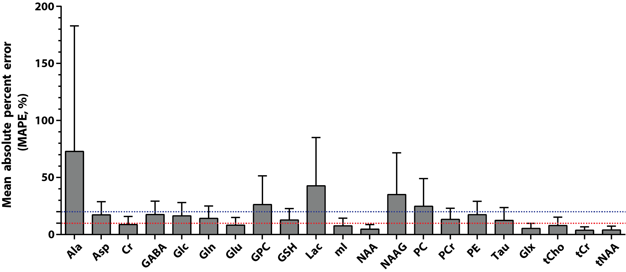
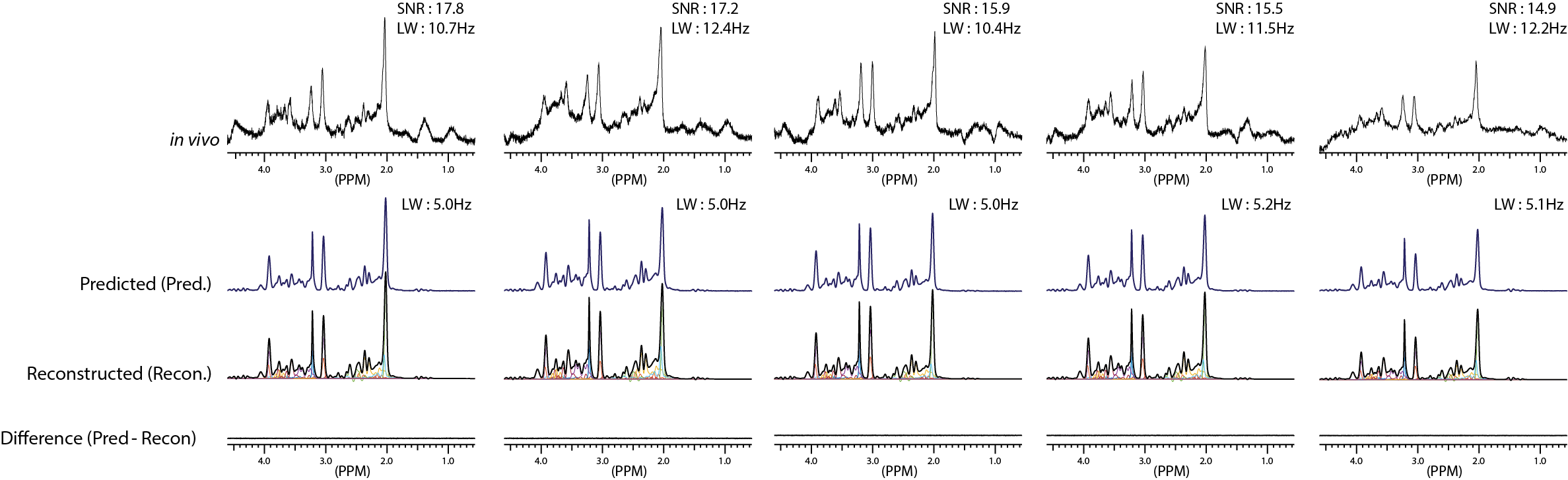
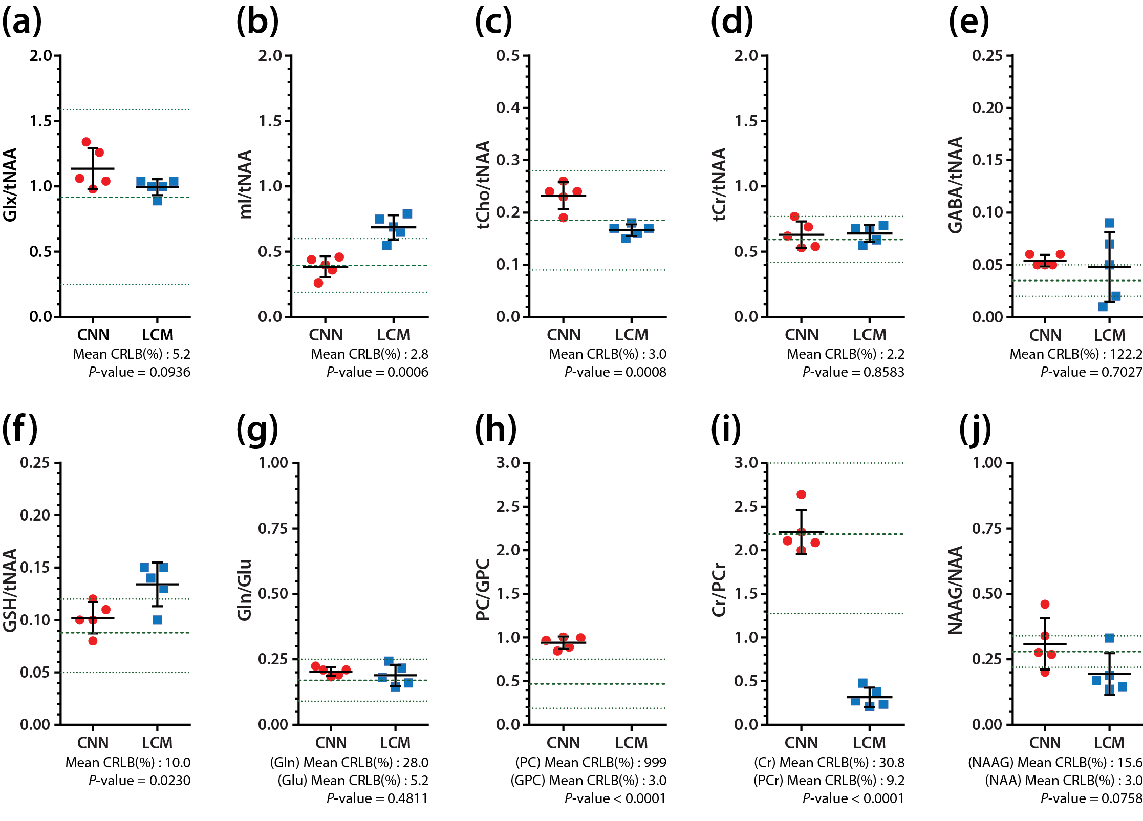
The representative simulated spectra in the test set are shown in Fig.2(a-d) along with the ground-truth (e-h) and the CNN-predicted metabolite-only spectra (i-l). The SNR and linewidth of tNAA ranged 7-21 and 10-20 Hz in the simulated spectra. The results of metabolite quantification using the proposed method are shown in Fig.3. Excluding Ala, GPC, Lac, NAAG and PC (MAPE>20%), MAPE was 12.49±4.35% for the rest of the metabolites over the whole simulated spectra in the test set. The in vivo spectra are shown for all volunteers in Fig.4, along with the CNN-predicted spectra. The capability of the CNN in removing the noise, line-broadening and baseline is clearly demonstrated. The results of metabolite quantification from the in vivo spectra using the proposed method and the LCModel analysis are compared in Fig.5 for those metabolites that are most commonly reported in the literature (a-d), challenging to detect (e-f), and difficult to separate from each other (g-j). The metabolite concentrations are within or close to the expected ranges from the literature except mI, GSH and especially Cr/PCr for the LCModel analysis and PC/GPC for both approaches.

Discussion

The difference spectra (Fig.3 and 4) demonstrate that the CNN fulfills its tasks of removing noise, line-broadening, phase/frequency shift, and baseline as trained such that the CNN-predicted spectra can be completely accounted for by a linear combination of the metabolite phantom spectra only. Whereas the typical in vivo SNR and linewidth of tNAA are >20 and ~10-12 Hz, they were 7-21 and 10-20 Hz in our simulated spectra. Nonetheless, a MAPE of 12.49±4.35% was achieved over the majority of the metabolites. Given the regional variations of metabolite concentrations, the deviation of mI and GSH from the expected concentration ranges with the LCModel analysis may need to be carefully interpreted. However, the estimated Cr/PCr value using the LCModel analysis was substantially deviated from the expected range (~1.3-3.0), ^18,19 which supports the efficacy of the line-narrowing provided by the proposed method.

Conclusion

Deep learning has a great potential for brain metabolite quantification in ¹H-MRS.

Acknowledgements

This research was supported by Basic Science Research Program through the National Research Foundation of Korea (NRF) funded by the Ministry of Education, Science and Technology (2016R1D1A1B03931233), by the Bio & Medical Technology Development Program of the NRF funded by the Korean government, MSIP (NRF-2014M3A9B6069340), by grant no 03-2016-0220 from the SNUH Research Fund, and by the Doosan Yonkang Foundation (30-2017-0120) in Korea.

References

1. Ratiney H, Coenradie Y, Cavassila S, et al. Time-domain quantitation of ¹H short echo-time signals: background accommodation. MAGMA. 2004;16(6):284–296

2. Provencher SW. Estimation of metabolite concentrations from localized in vivo proton NMR spectra. Magn Reson Med. 1993;30(6):672–679.

3. Bhogal AA, Schür RR, Houtepen LC, et al. ¹H-MRS processing parameters affect metabolite quantification: The urgent need for uniform and transparent standardization. NMR Biomed. 2017;30(11):e3804.

4. LeCun Y, Bengio Y, Hinton G. Deep learning. Nature. 2015;521(7553):436–444.

5. Pereira S, Pinto A, Alves V, et al. Brain tumor segmentation using convolutional neural networks in MRI images. IEEE Trans Med Imaging. 2016;35(5):1240–1251.

6. De Graaf RA. In vivo NMR spectroscopy: principles and techniques. John Wiley & Sons. 2007.

7. Govindaraju V, Young K, Maudsley AA. Proton NMR chemical shifts and coupling constants for brain metabolites. NMR Biomed. 2000;13(3):129–153.

8. Perry TL, Berry K, Hansen S, et al. Regional distribution of amino acids in human brain obtained at autopsy. J Neurochem. 1971;18(3): 513–519.

9. Perry TL, Berry K, Hansen S, et al. Free amino acids and related compounds in biopsies of human brain. J Neurochem. 1971;18(3): 521–528.

10. Birch R, Peet AC, Dehghani H, et al. Influence of macromolecule baseline on ¹H MR spectroscopic imaging reproducibility. Magn Reson Med. 2017;77(1): 34–43.

11. Opstad KS, Bell BA, Griffiths JR, et al. Toward accurate quantification of metabolites, lipids, and macromolecules in HRMAS spectra of human brain tumor biopsies using LCModel. Magn Reson Med 2008;60(5):1237–1242.

12. Gottschalk M, Lamalle L, Segebarth C. Short-TE localised ¹H MRS of the human brain at 3 T: Quantification of the metabolite signals using two approaches to account for macromolecular signal contributions. NMR Biomed. 2008;21(5):507–517.

13. Snoek J, Larochelle H, Adams RP. Practical bayesian optimization of machine learning algorithms. Adv Neural Inf Process Syst. 2012;pp 2951–2959.

14. Pouwels, PJ, Frahm J. Regional metabolite concentrations in human brain as determined by quantitative localized proton MRS. Magn Reson Med. 1998;39(1):53–60.

15. Ganji SK, An Z, Banerjee A, et al. Measurement of regional variation of GABA in the human brain by optimized point‐resolved spectroscopy at 7 T in vivo. NMR Biomed. 2014;27(10):1167–1175.

16. Kaiser LG, Schuff N, Cashdollar N, et al. Age-related glutamate and glutamine concentration changes in normal human brain: ¹H MR spectroscopy study at 4 T. Neurobiol Aging. 2005;26(5):665–672.

17. Komoroski RA, Pearce JM, Mrak RE. ³¹P NMR spectroscopy of phospholipid metabolites in postmortem schizophrenic brain. Magn Reson Med. 2008;59(3):469–474.

18. Hetherington HP, Spencer DD, Vaughan JT et al. Quantitative ³¹P spectroscopic imaging of human brain at 4 Tesla: Assessment of gray and white matter differences of phosphocreatine and ATP. Magn Reson Med. 2001;45(1):46–52.

19. Barker PB, Soher BJ, Blackband SJ, et al. Quantitation of proton NMR spectra of the human brain using tissue water as an internal concentration reference. NMR Biomed. 1993;6(1):89–94.

20. Choi C, Ghose S, Uh J, et al. Measurement of N‐acetylaspartylglutamate in the human frontal brain by ¹H‐MRS at 7 T. Magn Reson Med. 2010;64(5):1247–1251.

Figures

A schematic diagram of the simulation of brain spectra and the training of the convolutional neural network (CNN). The CNN was trained using a stochastic gradient descent with momentum algorithm. The loss function was mean-squared-error. The number of repetitions (n_rep) of the convolution-batch normalization-ReLU layers in the convolutional blocks was Bayesian-optimized together with the learning rate, momentum of the stochastic gradient descent algorithm, and L₂ regularization parameter. To mimic in vivo brain spectra the metabolite-only spectra are degraded with noise, line-broadening, frequency/phase shift, and spectral baseline. The CNN is trained to map the degraded brain spectra into noise-free, line-narrowed, frequency/phase shift-corrected, baseline-removed, metabolite-only spectra.

Representative simulated brain spectra in the test set and corresponding CNN-predicted spectra. (a)-(d): simulated brain spectra used as the input to the CNN. (e)-(h): ground-truth (GT) spectra simulated by linearly combining the metabolite phantom spectra. (i)-(l): CNN-predicted metabolite-only spectra (Pred.). (m)-(p): reconstructed spectra (Recon.) by linearly combining the metabolite phantom spectra according to the relative metabolite concentrations estimated from the CNN-predicted spectra. The metabolite phantom spectra used for the reconstruction are also shown. (q)-(t): difference spectra obtained by subtracting the CNN-predicted spectra from the ground-truth spectra (GT – Pred.). (u)-(x): difference spectra obtained by subtracting the reconstructed spectra from the CNN-predicted spectra (Pred. – Recon.).

Mean-absolute-percent-error (MAPE) in the concentrations of the metabolites estimated over all simulated brain spectra in the test set (N = 5000). The MAPE was estimated, first, by quantifying each individual metabolite from the CNN-predicted metabolite-only spectra by solving the inverse problem, and then, by comparing the estimated concentrations with the ground-truth concentrations.

In vivo brain spectra (in vivo) from the five healthy subjects and the corresponding CNN-predicted metabolite-only spectra (Pred.). The difference spectra (Pred – Recon) between the CNN-predicted metabolite-only spectra and the reconstructed spectra (Recon.) by linearly combining the metabolite phantom spectra according to the relative metabolite concentrations estimated from the CNN-predicted spectra demonstrate that the CNN successfully mapped the degraded in vivo spectra into the noise-free, line-narrowed, baseline-removed, metabolite-only spectra that can be completely accounted for by a linear combination of the metabolite phantom spectra only.

Comparison of the relative metabolite concentrations estimated by the proposed method (CNN) and the LCModel analysis (LCM) from the in vivo brain spectra (n=5). In the LCModel analysis, the PC/GPC values (h) were not available because the concentrations of PC were not detectable for all subjects. The mean metabolite concentrations estimated herein were marked with thick-solid lines. The corresponding standard deviations (SD) are shown together. The expected metabolite concentration ranges from the literature (mean±2SD) were marked with dotted lines (the mean values marked with thick-dotted lines). (References for the expected metabolite concentration ranges: Glx¹⁴, mI¹⁴, tCho¹⁴, tCr¹⁴, GABA¹⁵, GSH¹⁵, Gln/Glu¹⁶, PC/GPC¹⁷, Cr/PCr^18,19, and NAAG/NAA²⁰).

Proc. Intl. Soc. Mag. Reson. Med. 27 (2019)

1113