Synopsis

A new method to perform a multi-component analysis in MR Fingerprinting is proposed, which is faster and less sensitive to noise than previous methods. The algorithm finds a small number of components throughout the region of interest without assumptions about the number or relaxation times of the components. The proposed method is compared to previously published methods in numerical simulations and in vivo experiments.

Introduction

MR Fingerprinting(MRF) [1] is a new approach to quantitative MRI that uses a sequence of varying acquisition parameters to derive multiple tissue and system parameters in a single scan. When multiple tissues are present in a voxel, the measured signal is a linear combination of their signal evolutions. Previously proposed approaches to MRF multi-component analysis either use fixed components [2] or perform the analysis separately for each voxel [3,4], making it difficult to interpret the results over a larger region of interest. The practical application of the latter methods is additionally limited by long computation times reported to be 1-10s per voxel.

In this work, we introduce a computationally feasible method for MRF multi-component analysis that searches for components present in all voxels using a joint sparsity constraint, in addition to the common non-negativity constraints.

Methods

Instead of performing multi-component analysis for each voxel individually, we consider all voxels together. The main premise of the proposed approach is that the MRF signal can be represented as a linear combination of a few basis signals, corresponding to different components (e.g. myelin water, intra- and extra-cellular water, free water), and that these components are the same for all voxels.

This leads to the following minimization problem:$$\min_{\mathbf{C}\in \mathbb{R}_{\geq 0}^{N\times J}}\lVert \mathbf{X}-\mathbf{D}\mathbf{C}\rVert^2_F+\lambda\sum_{i=1}^N\lVert\mathbf{c}^i \rVert_0.$$Here $$$\mathbf{X}$$$ is a matrix containing the $$$J$$$ measured signals, $$$\mathbf{D}$$$ the MRF dictionary, each column of $$$\mathbf{C}$$$ contains the coefficients of the $$$N$$$ components for a voxel and $$$\mathbf{c}^i$$$ denotes the i^th row of $$$\mathbf{C}$$$. The parameter $$$\lambda$$$ balances the approximation error and the number of basis signals. The joint basis problem without non-negativity constraints has been studied extensively in distributed compressed sensing literature[5]–[9].

To solve this problem we propose a new algorithm, the Sparsity Promoting Iterative Joint NNLS(SPIJN) algorithm. The joint sparsity constraint is introduced by the weights $$$w_i=\lVert\mathbf{c}^i\rVert_2+\epsilon~(i=1,…,N)$$$ (here $$$\epsilon=10^{-4}$$$), which is the $$$\ell_2$$$-norm of the coefficients over the FOV. The core of each iteration is formed by the NNLS algorithm[10], which is used to solve the reweighted NNLS problem $$$\min_{\mathbf{C}\in\mathbb{R}_{\geq 0}^{N\times~J}}\lVert\tilde{\mathbf{X}}-\tilde{\mathbf{D}}\mathbf{C}\rVert^2_F$$$. Each iteration of the algorithm is given by:$$\mathbf{W}_{k+1}=\operatorname{diag}(\left(\mathbf{w}\right)_{k+1}^{1/2}),\\\tilde{\mathbf{D}}_{k+1}=\begin{bmatrix}\mathbf{D}\mathbf{W}_{k+1}\\\lambda\mathbf{1}^T\end{bmatrix},\\\tilde{\mathbf{X}}=\begin{bmatrix}\mathbf{X}_{k+1}\\\mathbf{0}^T\end{bmatrix},\\\tilde{\mathbf{C}}_{k+1}=\operatorname{argmin}_{\mathbf{C}\in\mathbb{R}_{\geq0}^{N\times~J}}\lVert\tilde{\mathbf{X}}-\tilde{\mathbf{D}}\mathbf{C}\rVert^2_F,\\\mathbf{C}_{k+1}=\mathbf{W}_{k+1}\tilde{\mathbf{C}}_{k+1}.$$ This method is compared to the NNLS algorithm [10], the reweighted $$$\ell_1$$$-method [4] and the Bayesian method[3]. A dictionary containing 3240 T₁/T₂ combinations was used, both sampled in 80 steps on a logarithmic scale from 10ms to 5s with the restriction $$$T_2\leq~T_1$$$.

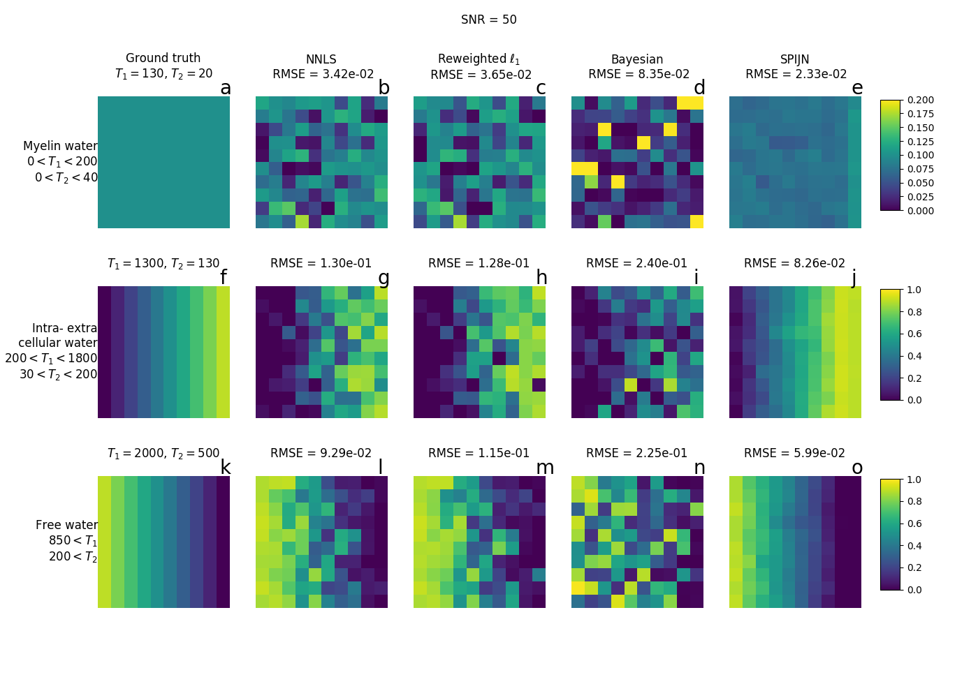
The methods were compared in numerical simulations and in vivo brain measurements with the sequence of[11] with length 200. The numerical simulations included three T₁/T₂ combinations; 1)T₁=130ms, T₂=20ms related to myelin water, 2)T₁=1300ms, T₂ =130ms related to intra- and extra-cellular water and 3)T₁=2000ms, T₂=500ms related to free water. Gaussian noise was added resulting in SNR=50.

Matched components are grouped using the following boundaries 1)T₁<200ms,T₂<40ms,2) 200ms<T₁<1800ms,30ms<T₂<200ms and 3)T₁>850ms,T₂>200ms.

For the in vivo comparison,multi-component analysis using three fixed components was also performed. The first set of components, as rough estimation, is taken from literature[2] and the second from the components found by SPIJN.

Results and discussion

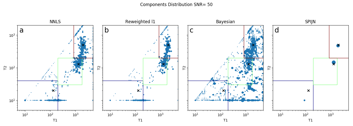
Fig.1,2 show results from the simulations. For all methods, the component with short T₂ is most difficult to estimate. This might indicate that the MRF-sequence is not very sensitive to T₂ in this range. The results for NNLS and reweighted-$$$\ell_1$$$ are very similar and show smaller error than the Bayesian method. The error is further reduced by the joint sparsity constraint used in the SPIJN algorithm.

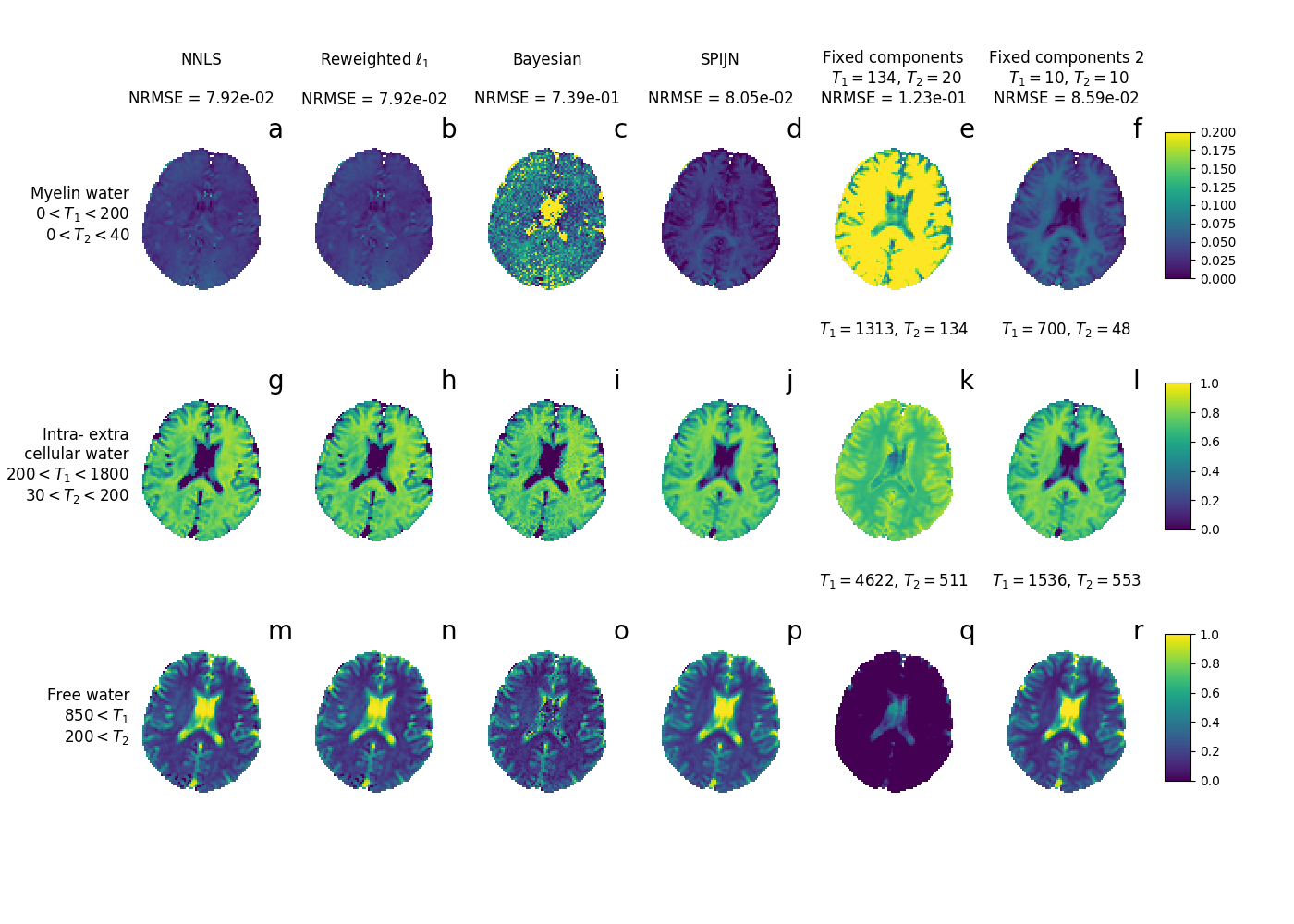
Fig.3,4 show results for the in vivo data. NNLS and reweighted-$$$\ell_1$$$ give exactly the same results, although NNLS is much faster.

The results using literature-based fixed components are very different, which shows the sensitivity to the chosen relaxation times. The approximation error is reduced when using fixed components based on the SPIJN algorithm, but still larger than for the complete dictionary algorithms.

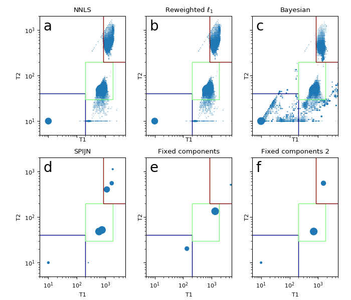
Only the SPIJN algorithm shows white-grey matter contrast in the myelin water component, for the other components the matching results are very similar, although the Bayesian approach shows some problems in the free water. The SPIJN algorithm shows smoother boundaries between the components, although no spatial regularisation is involved.

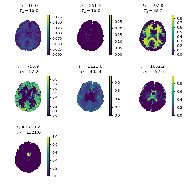
The 7 components matched by SPIJN are shown in Fig.5. The third and fourth component seem to resemble white and grey matter, although the T₁ values are shorter than expected. The meaning of the second and fifth component is unknown. The sixth and seventh component seem to represent CSF.

Conclusion

Acknowledgements

References

[1] D. Ma et al., “Magnetic resonance fingerprinting,” Nature, vol. 495, no. 7440, pp. 187–192, Mar. 2013.

[2] A. Deshmane et al., “Tissue Mapping in Brain Tumors with Partial Volume Magnetic Resonance Fingerprinting (PV-MRF),” in Proc. Intl. Soc. Mag. Reson. Med. 23, 2015, p. 0071.

[3] D. McGivney et al., “Bayesian estimation of multicomponent relaxation parameters in magnetic resonance fingerprinting: Bayesian MRF,” Magn. Reson. Med., Nov. 2017.

[4] S. Tang et al., “Multicompartment magnetic resonance fingerprinting,” Inverse Probl., vol. 34, no. 9, p. 094005, Sep. 2018.

[5] M. F. Duarte, S. Sarvotham, D. Baron, M. B. Wakin, and R. G. Baraniuk, “Distributed Compressed Sensing of Jointly Sparse Signals,” 2005, pp. 1537–1541.

[6] S. F. Cotter, B. D. Rao, Kjersti Engan, and K. Kreutz-Delgado, “Sparse solutions to linear inverse problems with multiple measurement vectors,” IEEE Trans. Signal Process., vol. 53, no. 7, pp. 2477–2488, Jul. 2005.

[7] J. A. Tropp, A. C. Gilbert, and M. J. Strauss, “Algorithms for simultaneous sparse approximation. Part I: Greedy pursuit,” Signal Process., vol. 86, no. 3, pp. 572–588, Mar. 2006.

[8] J. A. Tropp, “Algorithms for simultaneous sparse approximation. Part II: Convex relaxation,” Signal Process., vol. 86, no. 3, pp. 589–602, Mar. 2006.

[9] J. D. Blanchard, M. Cermak, D. Hanle, and Y. Jing, “Greedy Algorithms for Joint Sparse Recovery,” IEEE Trans. Signal Process., vol. 62, no. 7, pp. 1694–1704, Apr. 2014.

[10] C. L. Lawson and R. J. Hanson, Solving least squares problems. SIAM, 1974.

[11] M. Doneva, T. Amthor, P. Koken, K. Sommer, and P. Börnert, “Matrix completion-based reconstruction for undersampled magnetic resonance fingerprinting data,” Magn. Reson. Imaging, vol. 41, pp. 41–52, Sep. 2017.