Synopsis

This work extends the hybrid-state model, recently introduced to explain and optimize the dynamics of complex non-steady-state pulse sequences such as MR Fingerprinting, to magnetization transfer. We numerically optimize a hybrid-state pulse sequence for SNR efficiency and demonstrate the potential of the extended hybrid-state framework for quantification of MT effects in vivo in the human brain. Our preliminary results show good agreement with literature and demonstrate the feasibility of quantifying the fractional semi-solid pool size, as well as T1 and T2 relaxation times of the free pool, in under 10 minutes.

Introduction

Theory

The dynamics of free spins is commonly described by the Bloch equation. Assuming $$$T_R\ll\{T_1,T_2\}$$$ and assuming slow variations of the sequence parameters, such as the flip angle, all spin dynamics are captured by the radial component $$$r$$$ in spherical coordinates, which is controlled by the polar angle $$$\vartheta~$$$[1]. On-resonance, this polar angle is half the flip angle, which we will assume in the following.

Semi-solid spins, such as the ones bound in myelin, exhibit extremely short $$$T_2$$$ times and usually cannot be described by the Bloch equation$$$~$$$[2]. However, we can assume that their transversal magnetization vanishes, such that we can describe the entire dynamics of the semi-solid spin pool by its z-component. Under these assumptions, we can denote the standard two-pool model (one free pool indicated by the superscript $$$f$$$ and one semi-solid pool indicated by $$$s$$$)$$$~$$$[2] in hybrid state in a very compact form:$$\partial_t\begin{pmatrix}r^f\\z^s\\1\end{pmatrix}=\begin{pmatrix}-\frac{\cos^2\vartheta}{T_1^f}-\frac{\sin^2\vartheta}{T_2^f}-Rm_0^s&Rm_0^f\cos\vartheta&\frac{m_0^f\cos\vartheta}{T_1^f}\\Rm_0^s\cos\vartheta&-\frac{1}{T_1^s}-Rm_0^f-\bar{\eta}\vartheta^2&\frac{m_0^s}{T_1^s}\\0&0&0\end{pmatrix}\begin{pmatrix}r^f\\z^s\\1\end{pmatrix}.$$Here, the partial derivative with respect to time is denoted by $$$\partial_t$$$, the exchange rate between free and semi-solid spin pools by $$$R$$$, and the fractional proton densities of the semi-solid and free pool by $$$m_0^s$$$ and $$$m_0^f=1-m_0^s$$$, respectively. The saturation rate due of the semi-solid pool is given by $$$\bar{\eta}\vartheta^2$$$, which depends on $$$T_2^s$$$, the line shape of the semi-solid pool, the pulse shape, the duration of the RF-pulse $$$T_{RF}$$$, and $$$T_R$$$. For a Lorentzian line shape and rectangular pulses, the saturation rate is given by $$$\bar{\eta}=4T_2^s/(T_{RF}T_R)$$$. However, the model does not require knowledge of the line shape.

Methods

In the search for the most SNR-efficient hybrid-state MT sequence, we optimized $$$\vartheta$$$ and $$$T_{RF}$$$ as functions of time. We parameterized these functions as a sum of 100 Hann window functions over a span of $$$T_C=3$$$s and solved the ordinary differential equation shown above with a standard Runge–Kutta solver while ensuring anti-periodic boundary conditions ($$$r^f(0)=-r^f(T_C),z^s(0)=z^s(T_C)$$$)$$$~$$$[1]. We calculated the relative Cramer-Rao bound$$$~$$$[1,3,4] and minimized it numerically with the Broyden-Fletcher–Goldfarb-Shanno algorithm, while limiting $$$\pi/16\leq\vartheta\leq\pi,~T_{RF}\leq1$$$ms, and applying RF-amplitude and SAR limitations.

We tested the resulting sequence with an in vivo experiment at a 3T Prisma scanner (Siemens, Germany). Spatial encoding was performed with a sagittally oriented 3D stack-of-stars trajectory with golden angle increment$$$~$$$[6]. The spatial resolution is $$$1~\text{mm}\times1~\text{mm}\times 4~\text{mm}$$$ at a $$$FOV=256~\text{mm}\times256~\text{mm}\times192~\text{mm}$$$. The total scan time was $$$9.6~\text{min}$$$. Image reconstruction was performed with a low-rank ADMM approach$$$~$$$[5]. Due to computational limitations, we fixed $$$T_2^s=1\mu\text{s}$$$ and $$$T_1^s=1$$$s similar to Ref.$$$~$$$[7].

Results and Discussion

The numerical optimization results in comparably smooth $$$\vartheta$$$ and $$$T_{RF}$$$ patterns. $$$T_{RF}$$$ remains at the maximum duration during most parts of the sequence and thereby minimizes the saturation of the semi-solid pool (Fig.$$$~$$$1a,b). Only during three time periods does the optimization switch to the minimal pulse duration allowed by the RF-amplitude constraint. During this time, the semi-solid pool is saturated. When the z-components of the two pools differ, effective magnetization transfer occurs (cf.$$$~$$$Fig.$$$~$$$1a,d). The largest difference and, therefore, the largest magnetization transfer, occurs after the inversion pulse, which indicates that inversion recovery sequences are beneficial for quantitative MT imaging.

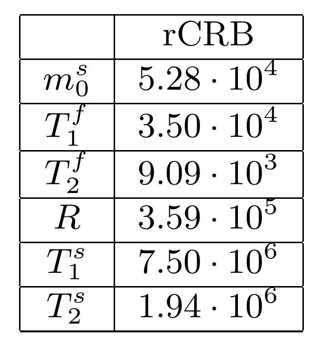
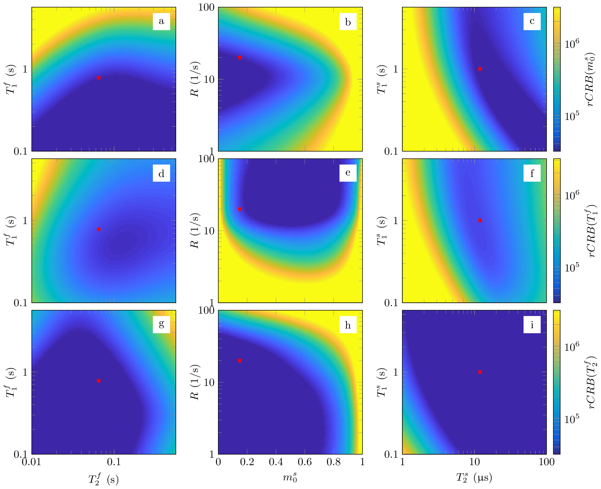
Our joint optimization for $$$m_0^s,T_1^f$$$, and $$$T_2^f$$$ results in significantly lower Cramer-Rao bounds for those values compared to the parameters that we did not optimize for ($$$R,T_1^s,T_2^s;~$$$Tab.$$$~$$$1). Fig.$$$~$$$2 demonstrates that these bounds translate comparable performance over large areas of the six-dimensional parameter space.

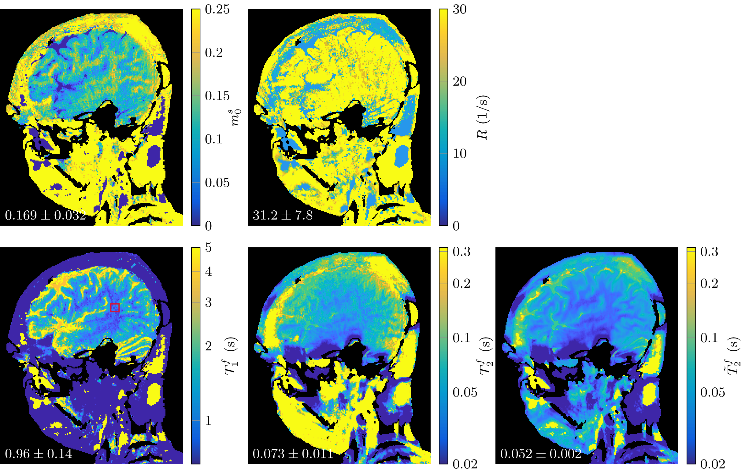
The in vivo parameter maps depicted in Fig.$$$~$$$3 demonstrate the feasibility of quantitative MT imaging in the hybrid state. A region-of-interest analysis in white matter agrees with literature within one standard deviation$$$~$$$[8]. Here, we define $$$T_2^f$$$ to purely quantify the relaxation within the free pool. Literature often uses the parameter $$$\tilde{T}_2^f=(1/T_2^f+Rm_0^s)^{-1}$$$ instead, i.e. one describes the entire decay of the transversal magnetization with $$$\tilde{T}_2^f$$$ (cf.$$$~$$$Fig.$$$~$$$3).

In order to fit the dictionary in the memory, we fixed $$$T_1^s=1$$$s and $$$T_2^s=1\mu$$$s. Our initial findings are that these parameters hardly influence the fit of the other parameters. Nonetheless, future work will include a fit of the entire model with a machine learning approach$$$~$$$[9,10], optimizations for the remaining model parameters, as well as a thorough validation and comparison to existing methods.

Acknowledgements

References

[1] Jakob Assländer, Dmitry S. Novikov, Riccardo Lattanzi, Daniel K. Sodickson, and Martijn A. Cloos. Hybrid-State Free Precession in Nuclear Magnetic Resonance. arXiv:1807:1–12, 2018.

[2] RM M Henkelman, X Huang, Q-S S Xiang, Greg J Stanisz, SD D Swanson, and MJ J Bronskill. Quantitative Interpretation of Magnetization Transfer. Magn. Reson. Med., 29(6):759–766, 1993.

[3] Harald Cramér. Methods of mathematical statistics. Princeton University Press, Princeton, NJ, 1946.

[4] Calyampudi Radhakrishna Rao. Information and the Accuracy Attainable in the Estimation of Statistical Parameters. Bull. Calcutta Math. Soc., 37(3):81–91, 1945.

[5] Jakob Assländer, Martijn A Cloos, Florian Knoll, Daniel K Sodickson, Jürgen Hennig, and Riccardo Lattanzi. Low rank alternating direction method of multipliers reconstruction for MR fingerprinting. Magn. Reson. Med., 79(1):83–96, 2018.

[6] Stefanie Winkelmann, Tobias Schaeffter, Thomas Koehler, Holger Eggers, and Olaf Doessel. An Optimal Radial Profile Order Based on the Golden Ratio for Time-Resolved MRI. IEEE Trans. Med. Imaging, 26(1):68–76, 2007.

[7] M Gloor, Klaus Scheffler, and Oliver Bieri. Quantitative magnetization transfer imaging using balanced SSFP. Magn. Reson. Med., 60(3):691–700, 2008.

[8] Greg J Stanisz, Ewa E Odrobina, Joseph Pun, Michael Escaravage, Simon J Graham, Michael J Bronskill, and R Mark Henkelman. T1,T2 relaxation and magnetization transfer in tissue at 3T. Magn Reson Med, 54(3):507–512, 2005.

[9] Gopal Nataraj, Jon-fredrik Nielsen, and Jeffrey A Fessler. DICTIONARY-FREE MRI PARAMETER ESTIMATION. In Proc. IEEEIntl. Symp. Biomed. Imag., pages 5–9, 2017.

[10] Ouri Cohen, Bo Zhu, and Matthew S. Rosen. MR fingerprinting Deep RecOnstruction NEtwork (DRONE). Magn. Reson. Med., 80(3):885–894, 2018.