1097
Convolutional neural network-based image reconstruction and image classification: atomization or amalgamation?1Weill Cornell Medicine, New York, NY, United States, 2Memorial Sloan Kettering Cancer Center, New York, NY, United States, 3Cornell University, Ithaca, NY, United States
Synopsis
Convolutional neural networks have emerged as a powerful tool for image reconstruction and image analysis. In this abstract, we evaluate whether image reconstruction and image classification tasks are best performed separately, or whether a combined CNN, performing image reconstruction and clinical diagnosis steps in tandem, delivers synergistic effects.
Introduction
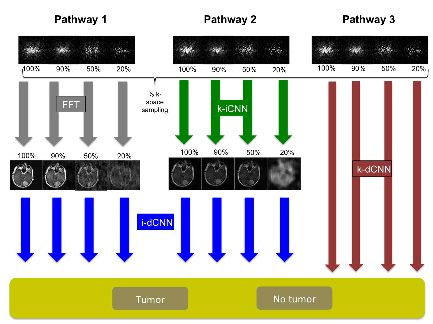
Convolutional neural networks(CNNs) are causing a paradigm shift in the way that MRI images are reconstructed and analyzed.1 Prior work has focused on developing CNNs for specific tasks, such as image reconstruction, image segmentation, or image classification. Our aim is to evaluate whether image reconstruction and image classification tasks are best performed by two separate CNNs, or whether a compound CNN, performing these steps in tandem, delivers synergistic effects. To that end, we designed three CNN pathways from k-space to diagnosis: (1) Fourier transform + image-space-to-diagnosis CNN(i-dCNN), (2) k-space-to-image-space CNN(k-iCNN) + image-space-to-diagnosis CNN(i-dCNN), and (3) k-space-to-diagnosis CNN(k-dCNN). We compared the performance of these three CNN pathways in a brain tumor detection task, using both fully-sampled and under-sampled artificially-generated k-space data.Methods
In this HIPPA-compliant, IRB-exempt study, a radiologist retrospectively identified 240 consecutive patients in our MRI database with enhancing tumors on post-contrast T1-weighted brain MRI. A second radiologist classified all slices as tumor-containing or not-tumor-containing. The superior-most and inferior-most tumor-containing slices were excluded due to partial volume effects. To maintain class balance, a subset of not-tumor-containing slices were randomly discarded. This yielded 1394 tumor-containing slices and 1403 non-tumor-containing slices.
Three
CNN pathways from k-space to diagnosis (i.e. “tumor” or “no tumor”) were
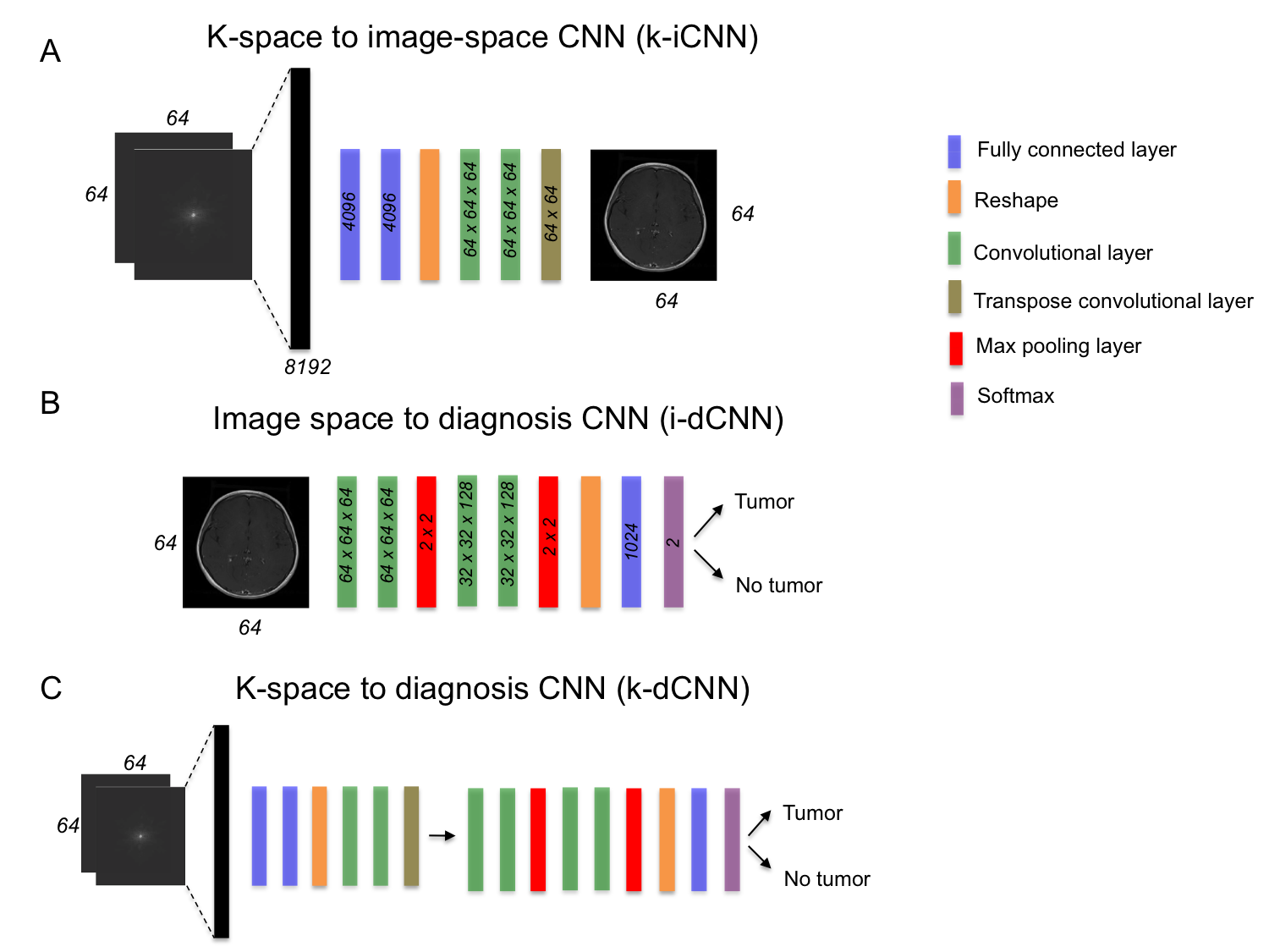
constructed. See Fig. 1 for a visual representation of the pathways and Fig. 2 for the CNN details.
Pathway 1 consisted of a Fourier transform followed by i-dCNN. The i-dCNN network architecture, a simplified version of VGG16,2 contained two sets of convolutional layers (3x3 filters) followed by rectified linear unit (ReLU) activation and max pooling, as well as a fully connected layer, 50% dropout,3 and softmax binary classification. The network was trained with a learning rate of 1e-3 for 20 epochs using the stochastic gradient descent optimizer.
Pathway 2 consisted of k-iCNN followed by i-dCNN. The k-iCNN architecture, data preprocessing, regularization parameters, and optimizer were taken from AUTOMAP.4 The network was trained with a learning rate of 1e-4 for 45 epochs. The i-dCNN was implemented the same way as in Pathway 1. This pathway separated the image reconstruction and image analysis tasks.
Pathway 3 contained k-dCNN, which is equivalent to k-iCNN + i-dCNN. The weights from this network were initialized with the weights from Pathway 2. The network was trained with a learning rate of 1e-6 for 20 epochs using the stochastic gradient descent optimizer. This pathway was designed to permit synergistic effects between image reconstruction and image analysis tasks.
The three CNN pathways were each trained four separate times, with the the network inputs containing varying extents of k-space sampling (i.e. 20%, 50%, 90%, 100%). All CNNs were designed in Python using Keras Toolbox and TensorFlow backend on a server and implemented with a NVIDIA GTX 1080ti GPU. All subjects were divided into training/validation/test groups by the ratio 80/10/10. The accuracy, sensitivity, specificity and AUC of each of the three CNN pathways were evaluated with various degrees of k-space sampling.
Results
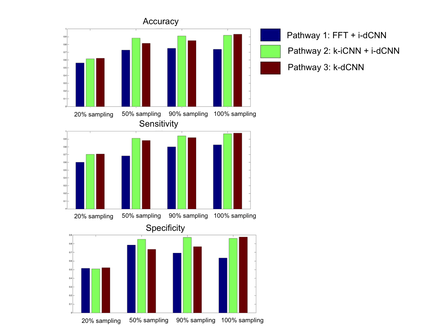
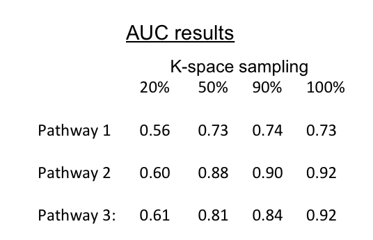
Figure 3 displays the accuracy, sensitivity, and specificity of all network classifications for all k-space sampling patterns. The AUCs are displayed in Figure 4. For all k-space sampling patterns, Pathway 2 (k-iCNN + i-dCNN) outperformed Pathway 1 (FFT + i-dCNN) and Pathway 3 (k-dCNN). For instance, at 50% k-space sampling, Pathway 2 accuracy, sensitivity, specificity and AUC were 0.88, 0.91, 0.85, and 0.88 respectively, while those of Pathway 3 were 0.72, 0.78, 0.68, and 0.73 respectively.Discussion
In this work, we demonstrate that Pathway 2 outperforms Pathway 1 and Pathway 3 for all degrees of k-space sampling. This suggests that, at least with present CNN designs, there are no synergistic gains in combining the reconstruction and classification tasks. We hypothesize that this is due, in part, to non-optimal permeation of k-space data through the network structure. CNNs use small filters to learn representations of data with increasing levels of abstraction -- first learning local patterns, then more global patterns. As such, CNNs are well-suited to decode image space content, which are characterized by a nested organization of patterns. But k-space lacks this underlying structure. The k-iCNN network circumvents this problem with a brute force approach of fully connected layers. To achieve synergy between image reconstruction and image classification, a more tailored approach that harnesses the intrinsic properties of k-space will be needed.Conclusion
Given present CNN designs, image reconstruction and image classification are best performed as distinct steps. No synergistic effects were observed by combining image reconstruction and image classification tasks. This may be due, in part, to the brute-force architecture of current CNN-based image reconstruction methods. This highlights the need to explore how to better design image reconstruction CNNs to harness the unique features of k-space.Acknowledgements
No acknowledgement found.References
1. Le Cun, Y, et al. Deep Learning. Nature. 2015; 521(7553):436-444.
2. Simonyan, K. & Zisserman, A. Very deep convolutional networks for large-scale image recognition. In Proc. International Conference on Learning Representationshttp://arxiv.org/abs/1409.1556 (2014).
3. Srivastava, N, et al. Dropout: A simple way to prevent neural networks from overfitting. Journal of Machine Learning Research. 2014. 15: 1929-1958.
Figures