1093
Active acquisition for MRI reconstruction1University of Florida, Gainesville, FL, United States, 2Facebook AI Research, Montreal, QC, Canada, 3NYU School of Medicine, New York, NY, United States
Synopsis
In this abstract, we introduce a novel pipeline for MRI reconstruction, which actively selects sampling trajectories in order to ensure high fidelity images, while speeding up the acquisition time. The pipeline is based on recent advances in deep learning and is composed of two networks interacting with each other in order to perform active acquisition. Results on a large scale knee dataset highlight the potential of the method when compared to standard acquisition heuristics. Moreover, we show that the learnt acquisition strategy efficiently reduces the reconstruction uncertainty and paves the way towards more applicable solutions for accelerating MRI.
Introduction
The main drawback of Magnetic Resonance Imaging (MRI) is its slow acquisition time, which can take up to one hour. Reducing the number of k-space measurements is a standard way of speeding up the examination time. However, images resulting from the undersampled k-space often exhibit blur or aliasing effects1, making them unsuitable for clinical use. Thus, the goal of MRI reconstruction is to restore a high fidelity image from partially observed measurements. This partial view naturally induces reconstruction uncertainty that can only be reduced by acquiring additional measurements.
Recently, Convolutional Neural Networks (CNNs) have shown excellent results in MRI reconstruction2. Typically, CNNs take as input a zero-filled image reconstruction and output a fully measured image reconstruction. It has been shown that this process works well when dealing with a fix set of k-space measurements defining a sampling trajectory2. However, fixing the sampling trajectory may lead to low quality reconstructions, depending on the difficulty of the cases. Therefore, we argue that the sampling trajectory should be adapted on the fly.Method
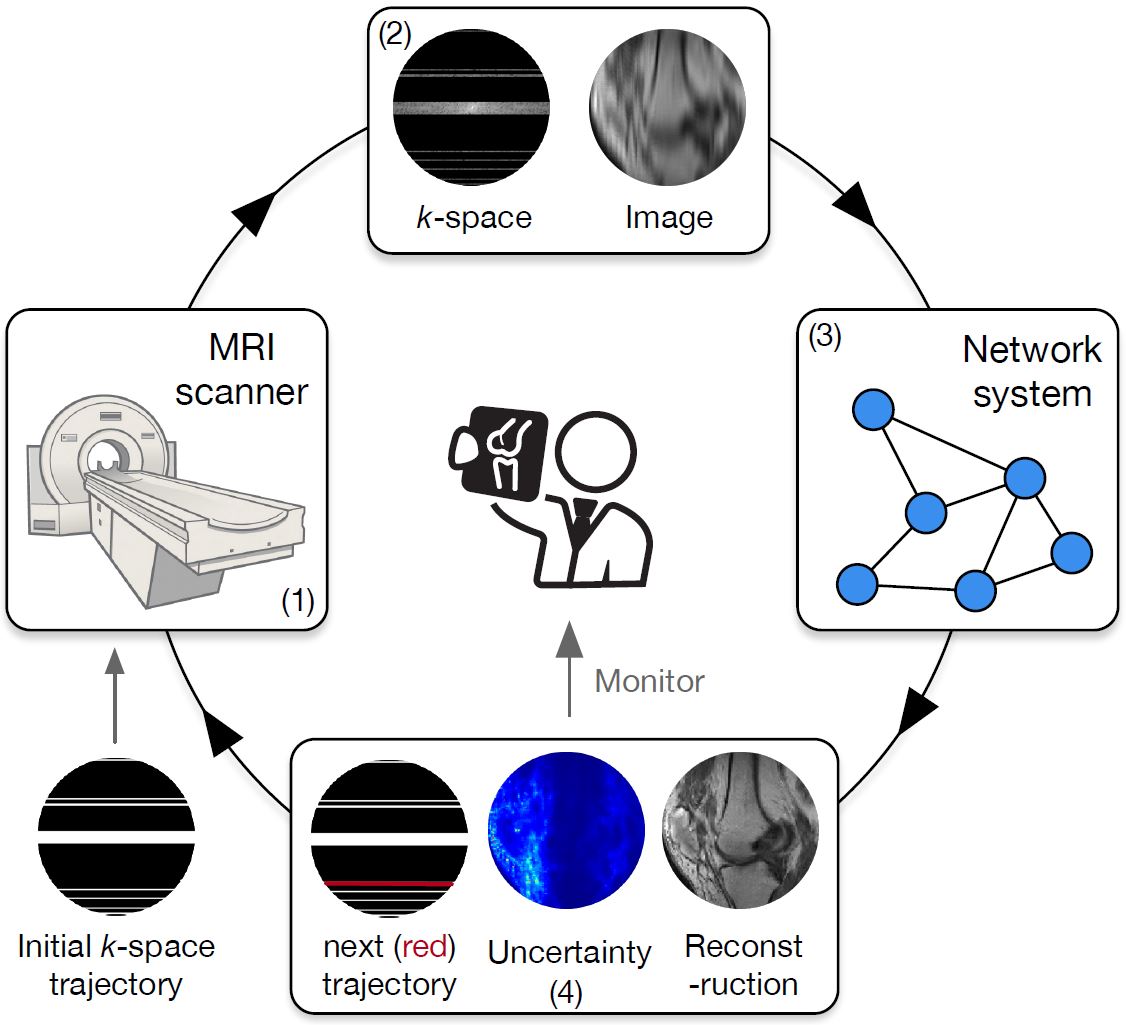
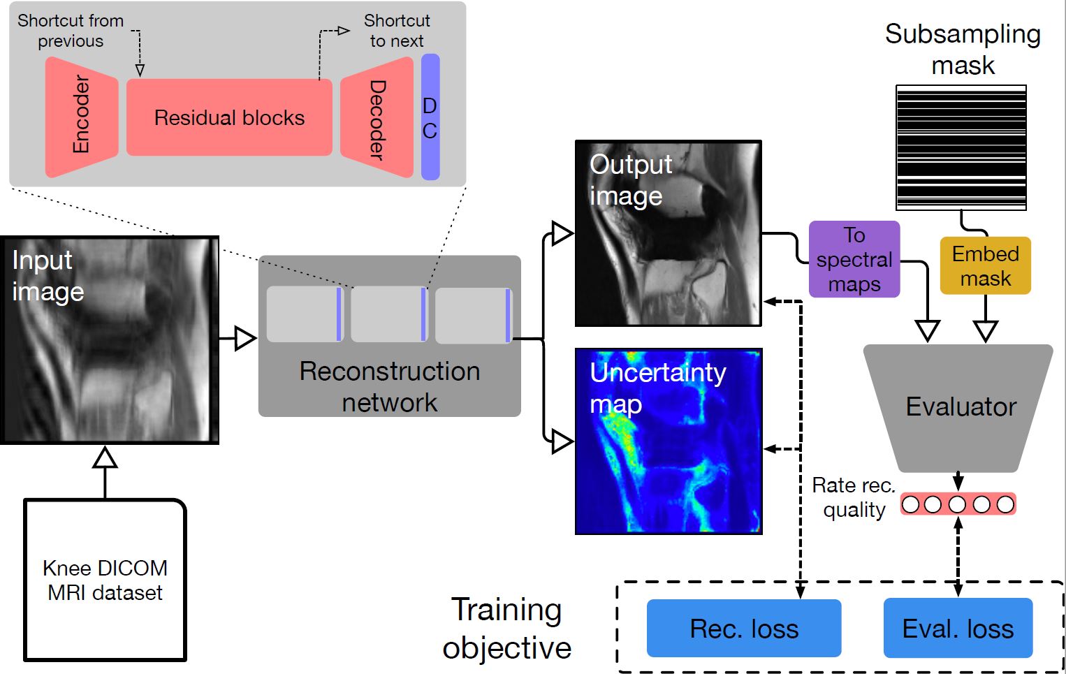
We present a novel pipeline for image reconstruction that dynamically tells the MRI scanner which measurements to acquire in order to best reduce the reconstruction uncertainty and, thus, its error. Figure 1 illustrates our system, which is driven by neural network advances3. The developed pipeline is composed of two networks interacting with each other. The first network, which has a cascaded backbone composed of fully convolutional ResNets (FC-ResNets)4,5 interleaved with data consistency layers2, aims to provide an image reconstruction together with pixel-wise uncertainty estimates. The second network aims to evaluate the quality of the reconstruction and drive the active acquisition by proposing the k-space trajectory to follow in order to reduce reconstruction uncertainty efficiently. To be proficient in this task, the network has to be able to capture small structural differences that define the distribution of the true, observed measurements. In our design, we leverage the idea of adversarial learning6,7 and train a modified discriminator to score the measurements, while encouraging the reconstruction network to produce results that match the true measurement distribution. Figure 2 depicts architectural details.
We use open sourced neural network library, PyTorch8, to develop and train our model.
Results
All experiments are conducted on a large scale Knee DICOM dataset, containing 11049 training images and 5048 test images. Among the training images, 10% are used for validation. All images are resized to have resolution 128x128. Volumes are from different machines and have different intensity range. We standardize each image using mean and standard deviation computed on the corresponding volume.
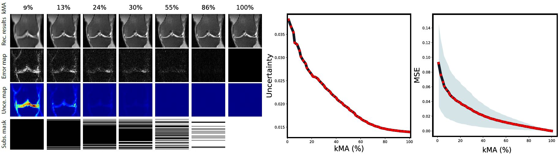
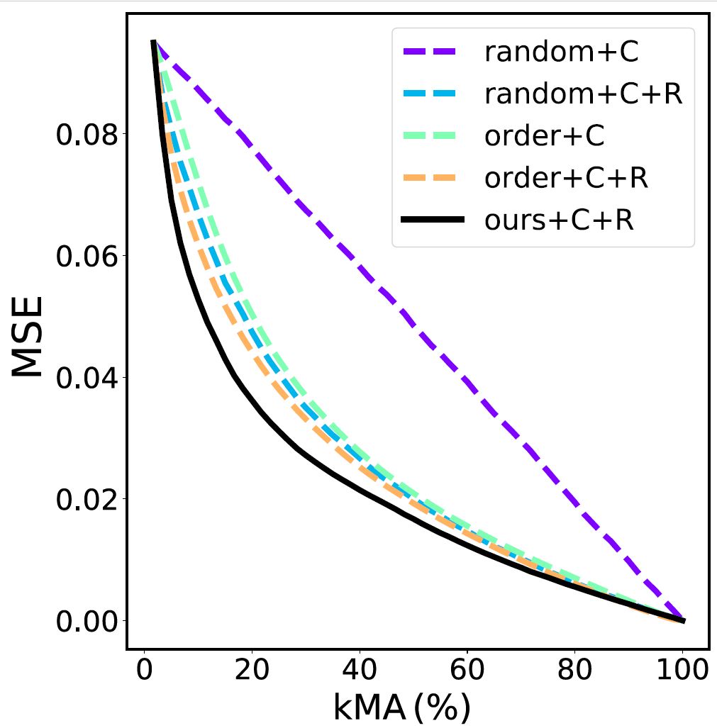
We simulate the active acquisition process of an MRI scanner. Given an input with a certain acquisition trajectory, we firstly obtain the reconstructed image. Then, we select the next unobserved row to acquire and measure it by copying it from the ground truth to the input image. After that, the updated input image is processed by our system. We iterate until the stopping criteria is met or the k-space is fully observed. The active acquisition process is depicted in Figure 3, which contains qualitative intermediate results at different k-space measurement ratios (kMA), i.e. the actual percentage of rows observed, including reconstructions, error maps, uncertainty estimates and acquisitions trajectories. The figure also outlines the progression of the mean uncertainty score and MSE on the test set. As shown in the figure, as we introduce additional measurements, the reconstruction quality improves and the error and uncertainty decrease. Moreover, higher uncertainty regions appear to have higher reconstruction error values.We compare our active acquisition system to several baselines by computing the MSE as a function of kMA (see Figure 4). We note that all methods have the same initial MSE and end up with zero error after observing all measurements. Random+C+R outperforms random+C remarkably, highlighting the benefit of applying the reconstruction network. However, order+C (even without any reconstruction) performs on par with random+C+R. This is not surprising, given that low frequency contains most of the information needed to reduce MSE. Finally, our method exhibits higher measurement efficiency when compared to the baselines.Conclusion
The promising results on the large knee dataset demonstrate that our method is effective and paves the road towards more applicable solutions for accelerating MRI, which ensure the optimal acquisition speedup while maintaining high fidelity image reconstructions with low uncertainty.Acknowledgements
The authors would like to thank Mary Bruno, Aaron Defazio, Krzysztof Geras, Joe Katsnelson, Florian Knoll, Yvonne Lui, Matthew Muckley, Erich Owens, Joelle Pineau, Michael Rabbat, Michael Recht, Daniel Sodickson, Anuroop Sriram, Mark Tygert, Nafissa Yakubova, Jure Zbontar, and Larry Zitnick for useful discussions and support.
References
1. D. Moratal, A. Valles-Luch, L. Marti-Bonmati, and M. E. Brummer. k-space tutorial: an mri educational tool for a better understanding of k-space. Biomedical imaging and intervention journal, 4(1), 2008.
2. J. Schlemper, J. Caballero, J. V. Hajnal, A. N. Price, and D. Rueckert. A deep cascade of convolutional neural networks for dynamic mr image reconstruction. IEEE transactions on Medical Imaging, 37(2):491–503, 2018.
3. LeCun, Y., Bengio, Y. & Hinton, G. Deep learning. nature 521, 436 (2015).
4. K. He, X. Zhang, S. Ren, and J. Sun. Deep residual learning for image recognition. In Proceedings of the IEEE conference on computer vision and pattern recognition, pages 770–778, 2016.
5. M. Drozdzal, E. Vorontsov, G. Chartrand, S. Kadoury, and C. Pal. The importance of skip connections in biomedical image segmentation. CoRR, abs/1608.04117, 2016.
6. I. Goodfellow, J. Pouget-Abadie, M. Mirza, B. Xu, D.Warde-Farley, S. Ozair, A. Courville, and Y. Bengio. Generative adversarial nets. In Advances in neural information processing systems, pages 2672–2680, 2014
7. A. Radford, L. Metz, and S. Chintala. Unsupervised representation learning with deep convolutional generative adversarial networks. CoRR, abs/1511.06434, 2015.
8. A. Paszke, S. Gross, S. Chintala, G. Chanan, E. Yang, Z. De-Vito, Z. Lin, A. Desmaison, L. Antiga, and A. Lerer. Auto-matic differentiation in pytorch. 2017
Figures