Synopsis

Magnetic resonance imaging (MRI) is an important but relatively slow imaging modality. MRI scan time can be reduced by undersampling the data and reconstructing the image using techniques such as compressed sensing or deep learning. However, the optimal undersampling pattern with respect to image quality and image reconstruction technique remains an open question. To approach this problem, our goal is to use reinforcement learning to train an agent to learn an optimal sampling policy. The image reconstruction technique is the environment and the reward is based upon an image metric.

Introduction

Non-linear reconstruction techniques such as compressed sensing and deep learning can reconstruct high quality images from undersampled data but an open question remains of how to determine an optimal undersampling pattern for these non-linear techniques, with respect to a given metric¹. Current heuristics for variable-density sampling emphasize sampling k-space center more than outer k-space. One approach to address this idea by Knoll et al. used an image dataset to learn and optimize a prior distribution².

In this work, we propose to find an optimal undersampling trajectory online using reinforcement learning (RL). Our hypothesis is that as data are collected, the agent may continuously infer the next best data to sample.

Methods

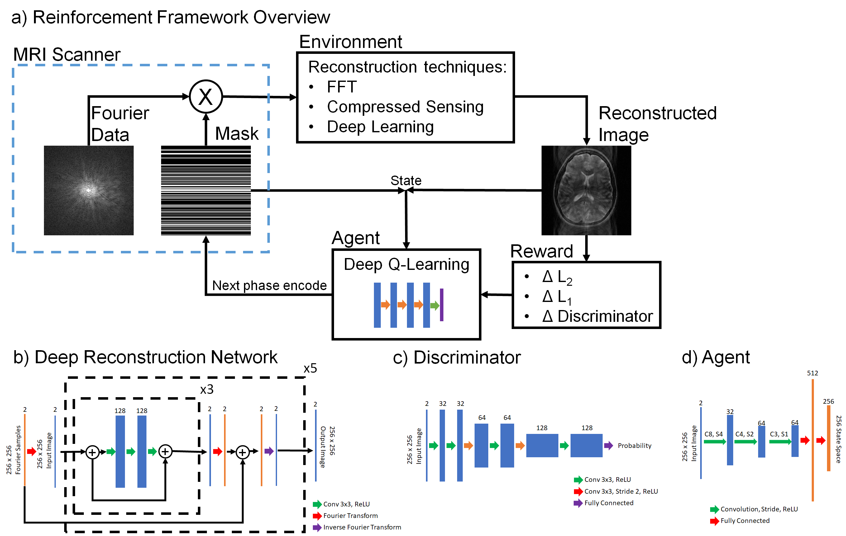
We used a set of ten fully-sampled, 3D knee datasets from mridata.org³ for a total of 3,840 2D images cropped to 256 x 256. We trained a deep Rainbow Q-learning⁴ agent to select the Cartesian phase encodes to sample (Figure 1).

The reinforcement learning environment was an image reconstruction technique. A Fourier transform was the baseline technique. For a compressed sensing reconstruction, we used L1-ESPIRiT with total variation regularization⁵. For deep reconstruction, we trained a generative adversarial network^6,7 (Figure 1) . The generator for reconstructing the image was an unrolled optimization network trained with a supervised L1 loss^8,9. The discriminator was a six-layer convolutional network.

The reinforcement learning reward was an image metric. All rewards were defined by subtracting the metric between the current step and the previous step. The metrics were L₂, L₁, and negative probability of the discriminator.

Our agent was a three-layer network with two fully connected layers¹⁰ (Figure 1d). The action state space was of size 256, representing the 256 potential readouts to sample, and encoded with ones to represent already-sampled readouts. The state for the agent was a row vector of the current action space and the current reconstructed image.

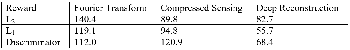
Nine agents were trained, for every combination of environment and reward. As a benchmark to evaluate the learned policies, the average number of readouts required to achieve less than 0.5% reward was determined over 100 episodes. 0.5% reward was chosen as a stopping point, based upon initial results to achieve an undersampling factor of about two to three.

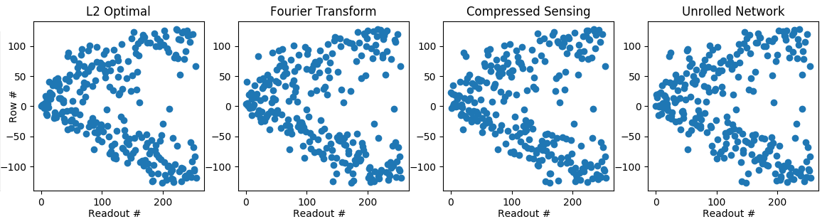
We further investigated the L₂ reward because Parseval’s Theorem allows us to determine the true optimal order of readouts in polynomial time. The baseline technique used only a learned prior distribution and was compared against the learned policies for all three reconstruction techniques.

Results

From the results in Figure 2, the compressed sensing and deep reconstruction techniques required fewer readouts than the Fourier transform reconstruction for the L₂ and L₁ rewards. This makes sense because the former two techniques are designed to infer data from undersampled raw data. The compressed sensing reconstruction required more readouts than the Fourier transform reconstruction for the discriminator metric, which may be because the discriminator is unfamiliar with compressed sensing artifacts.

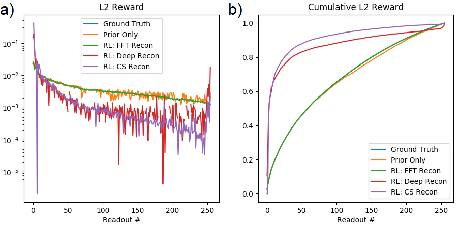
Figure 3 shows the learned policy and Figure 4 shows the reward per readout and cumulative reward as a function of policy. The ground truth L₂ policy and the learned policy for the Fourier transform reconstruction are nearly identical, such that it is difficult to distinguish the two in Figure 4. The policy using only prior-learned information was less consistent in choosing the best sample. Thus, in this instance where the solution is known, the reinforcement learning agent using online information outperformed the agent using only prior information.

Both compressed sensing and deep reconstructions acquired reward more quickly, echoing the results in Figure 3. We hypothesize that the deep reconstruction acquired reward more slowly than the compressed sensing because the deep reconstruction was trained with an L₁ loss.

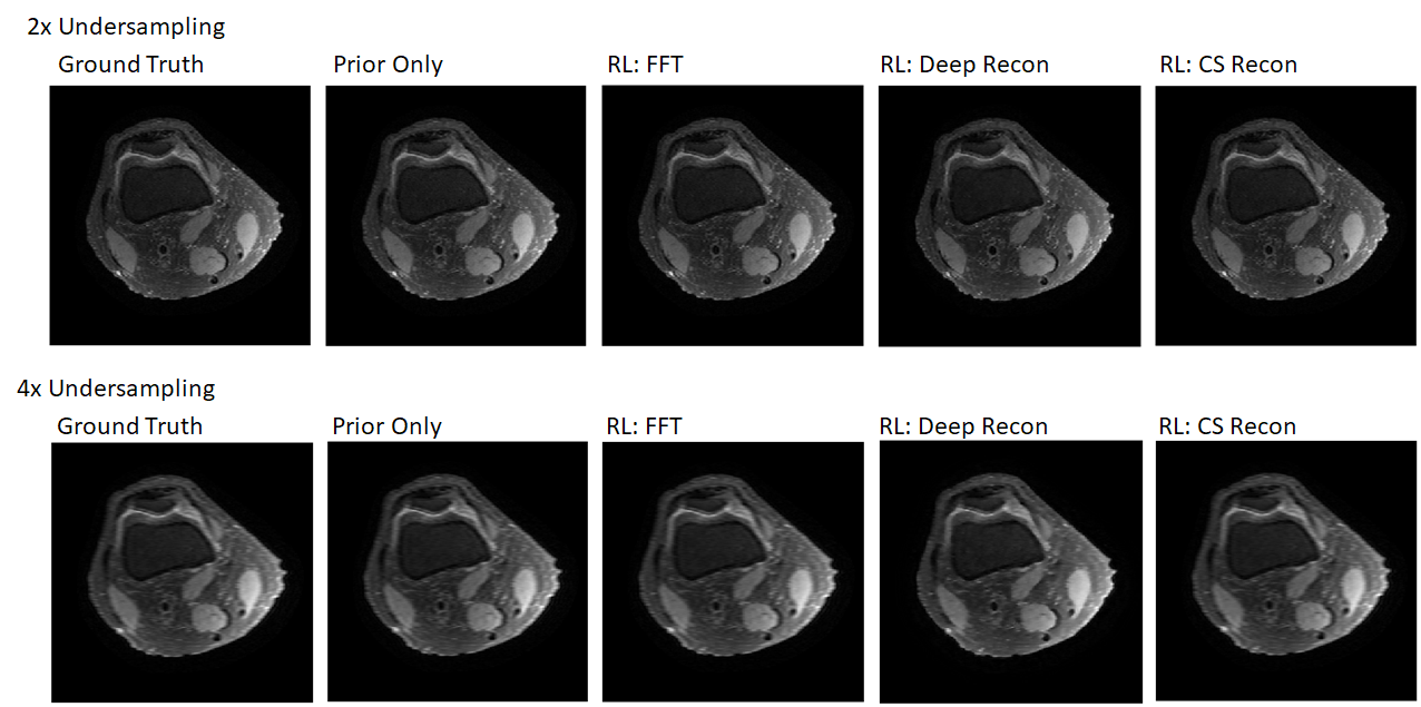
With the same policies, images at 2x and 4x undersampling were reconstructed (Figure 5). The images all look similar because L₂ only approximately captures image quality.

Discussion

Initial results of the reinforcement learning framework demonstrate feasibility and nearly optimal results, as verified by the L₂ reward results. Further analysis is required to understand the learned policies for other rewards and environments, which do not have solutions as accessible. The results highlight the inability of the L₂ reward to capture image quality. This raises motivation for the development of image quality metrics better aligned with diagnostic quality, which could then be addressed by the reinforcement learning framework.

We show results for optimization of 2D Cartesian sampling but for further generality we have formulated the problem as choosing the next readout, such that the framework can accommodate non-Cartesian and higher dimensional trajectories as well.

Acknowledgements

References

1. Lustig M, Donoho D, Pauly JM. Sparse MRI: The application of compressed sensing for rapid MR imaging. Magn. Reson. Med. 2007;58(6):1182–1195.

2. Knoll F, Clason C, Diwoky C, Stollberger R. Adapted random sampling patterns for accelerated MRI. MAGMA. 2011;24(1):43–50.

3. Epperson K, Sawyer A, Lustig M, Alley M, Uecker M. Creation of Fully Sampled MR Data Repository for Compressed Sensing of the Knee. In: Proceedings of the 22nd Annual Meeting for Section for Magnetic Resonance Technologists. 2013.

4. Hessel M, Modayil J, van Hasselt H, Schaul T, Ostrovski G, Dabney W, Horgan D, Piot B, Azar M, Silver D. Rainbow: Combining Improvements in Deep Reinforcement Learning. arxiv: 1710.02298. 2017 Oct 6.

5. Uecker M, Lai P, Murphy MJ, Virtue P, Elad M, Pauly JM, Vasanawala SS, Lustig M. ESPIRiT-an eigenvalue approach to autocalibrating parallel MRI: Where SENSE meets GRAPPA. Magn. Reson. Med. 2014;71(3):990–1001.

6. Mardani M, Gong E, Cheng JY, Vasanawala SS, Zaharchuk G, Xing L, Pauly JM. Deep Generative Adversarial Neural Networks for Compressive Sensing (GANCS) MRI. IEEE Trans. Med. Imaging. 2018:1–1.

7. Goodfellow IJ, Pouget-Abadie J, Mirza M, Xu B, Warde-Farley D, Ozair S, Courville A, Bengio Y. Generative Adversarial Networks. arxiv: 1406.2661. 2014 Jun 10.

8. Diamond S, Sitzmann V, Heide F, Wetzstein G. Unrolled Optimization with Deep Priors. 2017 May 22.

9. Cheng JY, Mardani M, Alley MT, Pauly JM, Vasanawala SS. DeepSPIRiT: Generalized Parallel Imaging using Deep Convolutional Neural Networks. In: Proceedings of ISMRM. 2018. p. 570.

10. Mnih V, Kavukcuoglu K, Silver D, Rusu AA, Veness J, Bellemare MG, Graves A, Riedmiller M, Fidjeland AK, Ostrovski G, et al. Human-level control through deep reinforcement learning. Nature. 2015;518(7540):529–533.