1069
About the need for a comprehensive description of the macromolecular baseline signal for MR fingerprinting and multidimensional fitting of MR spectra1University of Bern, Departments of Radiology and Biomedical Research, Bern, Switzerland, 2NIH, NIMH, Magnetic Resonance Spectroscopy Core, Bethesda, MD, United States
Synopsis
The purpose of this study was to evaluate the need for a comprehensive description of the macromolecular baseline signal (MMBL), e.g. for MR fingerprinting and multidimensional fitting of MR spectra. Inherent J-evolution for certain signals as well as multi-component T2-decays can cause variance of the signal shape as function of TE that is not described in a mono-exponential decay model. Two methods are described to accommodate this signal behavior when fitting a 2DJ-Inversion-Recovery dataset. In addition, the MMBLs for different TEs, as well as resulting metabolite contents, T1s and T2s with the conventional and alternative methods are reported.
Introduction
The definition of the macromolecular baseline (MMBL) underlying the metabolite resonances is one of the major challenges for quantification in clinical 1H Magnetic Resonance Spectroscopy (MRS). For quantification of brain spectra, recorded with a specific localization sequence at a certain echo (TE) and repetition time (TR), it is sufficient to know the specific MMBL signal intensities for that case. Various methods for the determination of such MMBLs have been suggested1. However, when preparing a dictionary for MR fingerprinting or when fitting a multidimensional dataset acquired under conditions involving different evolution periods of longitudinal and transverse magnetization2,3,4, a more comprehensive picture of the MMBL as a function of e.g. TE, TR and inversion time (TI) is needed. Here, we investigate the case of simultaneous fitting of a 2DJ-Inversion-Recovery (2DJIR) dataset with different combinations of TE and TI. Iterative procedures and simultaneous fitting of the whole dataset have been shown to allow determination of metabolite contents, T1 and T2 relaxation times at the same time as defining the MMBL as modeled by mono-exponentially decaying signals as function of TE. We investigate whether this condition should be relaxed to allow unconditioned variance of the signal shape as function of TE to accommodate inherent J-evolution5 as well as multi-component T2-decays. We report resulting MMBLs for different TEs, as well as resulting metabolite contents, T1s and T2s with the conventional and extended MMBL models.
Methods
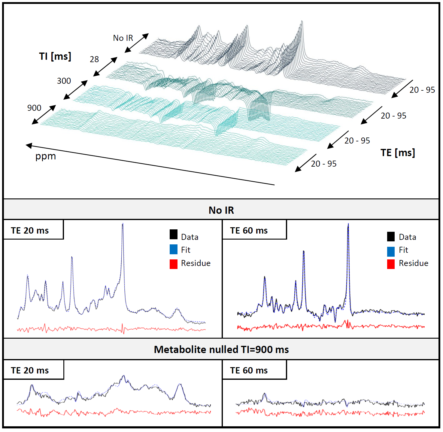
10 healthy volunteers, Siemens Trio 3T, quadrature headcoil; 2DJIR from inversion-prepared PRESS sequence (metabolite cycling, 64 scans per TE/TI combination, TR 3000-4000ms; ROI 28x28x20mm3). Data processing in MATLAB and jmrui6; present focus on summed spectra from all volunteers.
Interrelated datasets fitted with FiTAID3 including 18 metabolites and a MMBL model of 64 equally spaced lines (∆=0.05ppm, 0.7-4.1ppm), fixed Gaussian broadening: 5Hz; starting Lorentzian broadening: 15Hz, assigned to different groups after a first fit to allow component specific T1s and T2s for each group. Metabolite patterns simulated using real shaped pulses in GAMMA7,8,9. T1s and T2s were allowed to vary for metabolite sub-patterns.
The MMBL was modeled in three ways:
1. Mono-exponential model (MEM): All areas of the MMBL lines and grouped T1s and T2s fitted along with the metabolites for all spectra in the dataset (excl. TE>60ms at TI=900ms) with unmodified full TE-IR model.
2. Additional TE variation starting from MEM model: Keeping T1, T2 and metabolites fixed and fitting only the areas of the 64 MMBL lines separately at each TE<65 ms.
- Method A: Including all IR $$$\rightarrow$$$ 4x64=256 free parameters per TE
- Method B: Including only metabolite-nulled IR $$$\rightarrow$$$ 1x64=64 free parameters per TE
Then for A and B, the MMBL results for all TEs copied to the full model preserving their amplitude ratios between all TEs and the whole dataset fitted again in simultaneous mode.
Results and Discussion
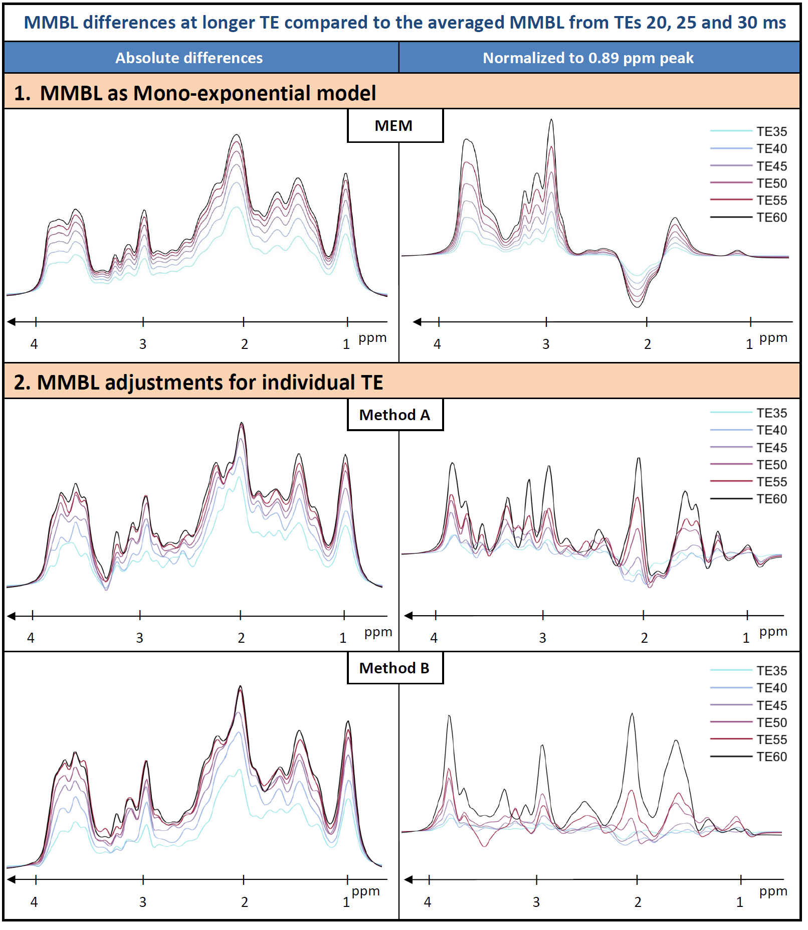
Figure 1 shows the initial adaptation of the MMBL in model MEM. Figure 2 gives an illustration of the complete dataset and representative fit results for method MEM. Figure 3 demonstrates the results for the MMBL from MEM as well as the new methods. Baseline variations caused by allowing the MMBL to adjust for each TE were detected for both cases. Figure 4 highlights some of these adaptations as differences for longer TE vs. short TE illustrating the changes in the MMBL with TE that are not described by mono-exponential relaxation. In Figure 5 preliminary results for concentrations as well as T1’s and T2’s for all metabolites are given for the three models of MMBL. As not all relaxation times could be fitted in the predefined ranges, differences in concentration vs. literature values may be caused by biased relaxation times. It is questionable whether a simultaneous quantification of T1, T2 and concentration of this many metabolite groups and MMBL with an as complex model as presented here is stable. To prevent overfitting, it may be preferable to restrain the fitting ranges or reduce the number of fit variables by assumed relations.Conclusions
Distinct MMBLs for different TEs, as well as resulting metabolite contents, T1s and T2s with the conventional and two alternative methods, were reported. The difference between the methods illustrates that the traditionally used mono-exponential decay model is not appropriate to represent J-evolution and multi-component T2-decays. In addition, insight into the challenges with simultaneous fitting of both metabolite and MMBL content as well as relaxation times is given ‑ suggesting that an inherently incorrect fit model with assumed (but not truly founded) prior knowledge may provide more robust and realistic results. Higher SNR data from higher fields may resolve some of the issues.Acknowledgements
This work is supported by the Swiss National Science Foundation (SNSF #320030‐175984).References
- Cudalbu et al., Handling Macromolecule Signals in the Quantification of the Neurochemical Profile. Journal of Alzheimer’s Disease (2012) 31: 101-115
- Bolliger et al., Modeling of 3-dimensional MR spectra of human brain: Simultaneous determination of T1, T2 and concentrations based on combined 2DJ inversion-recovery spectroscopy. Proc Intl Soc Mag Reson Med (2010) 18: #3325
- Chong et al., Two-dimensional linear-combination model fitting of magnetic resonance spectra to define the macromolecule baseline using FiTAID, a Fitting Tool for Arrays of Interrelated Datasets. Magn Reson Mater Phy (2011) 24: 147-164
- An et al., Simultaneous Determination of Metabolite Concentrations, T1 and T2 Relaxation Times. Magn Reson Med (2017) 78: 2072-2081
- Behar et al., Analysis of macromolecule resonances in 1H NMR spectra of human brain. Magn Reson Med (1994) 32: 294-302
- Stefan et al., Quantitation of magnetic resonance spectroscopy signals: the jMRUI software package. Measurement Science & Technology (2009) 20: 104035
- Smith et al., Computer Simulations in Magnetic Resonance. An Object-Oriented Programming Approach. J Magn Reson (1994) 106: 75-105
- https://scion.duhs.duke.edu/vespa/gamma/
- Hoefemann et al., Quantitative evaluation of systematic bias in clinical MRS introduced by the use of metabolite basis sets simulated with ideal RF pulses. Proc. Intl. Soc. Mag. Reson. Med. (2018) 26: #1313
Figures