1018
Comparison of Tumor Water Exchange Rate and Intracellular Water Lifetime Measured by Diffusion MRI1Radiology, New York University School of Medicine, New York, NY, United States
Synopsis
In vivo measurement of cellular-interstitial water exchange rate remains non-trivial. Its development is also hampered by the lack of a gold standard method for validation. In this study, we have used two complementary diffusion MRI methods to measure the water exchange rates. Time-dependent diffusional kurtosis imaging was used to measure the water exchange rate ($$$\tau_{ex}$$$) between the intra- and extra-cellular spaces, while a constant gradient diffusion MRI experiment was used to measure the intracellular water lifetime ($$$\tau_i$$$). These two measurements were conducted using GL261, a mouse glioma tumor model.
Introduction
In vivo measurement of cellular-interstitial water exchange rate remains non-trivial. Its development is also hampered by the lack of a gold standard method for validation. Diffusion MRI (dMRI) is a unique in vivo imaging technique sensitive to cellular microstructure at the scale of water diffusion length on the order of a few microns, such as cell size, cell density, composition of the extracellular matrix, compartmental diffusivities as well as water exchange between compartments.1,2 Diffusivity D, as well as higher-order dMRI metrics including diffusional kurtosis K, can reflect these tissue properties when measured with multiple diffusion times. The purpose of this study is to use two complementary dMRI methods to measure cellular-interstitial water exchange rates and compare them for cross-validation. Using GL261, a mouse glioma model, we measured the cellular-interstitial water exchange time ($$$\tau_{ex}$$$) in tumor tissue using time-dependent diffusion kurtosis imaging (tDKI), and compared that with the intracellular water lifetime ($$$\tau_i$$$) measured in the same tumors using constant gradient diffusion weighted imaging (CG-DWI) experiments.3Methods
Six-to-eight week old C57BL6 mice with GL261 glioma tumor model (n = 6) were included in this study performed using a Bruker 7T micro-MRI system with a four-channel phased array cryogenically-cooled receive-only coil with a volume-transmit coil. The animal body temperature was maintained at 36 ± 1 ºC during the scan. General anesthesia was induced by 1.5% isoflurane in air.
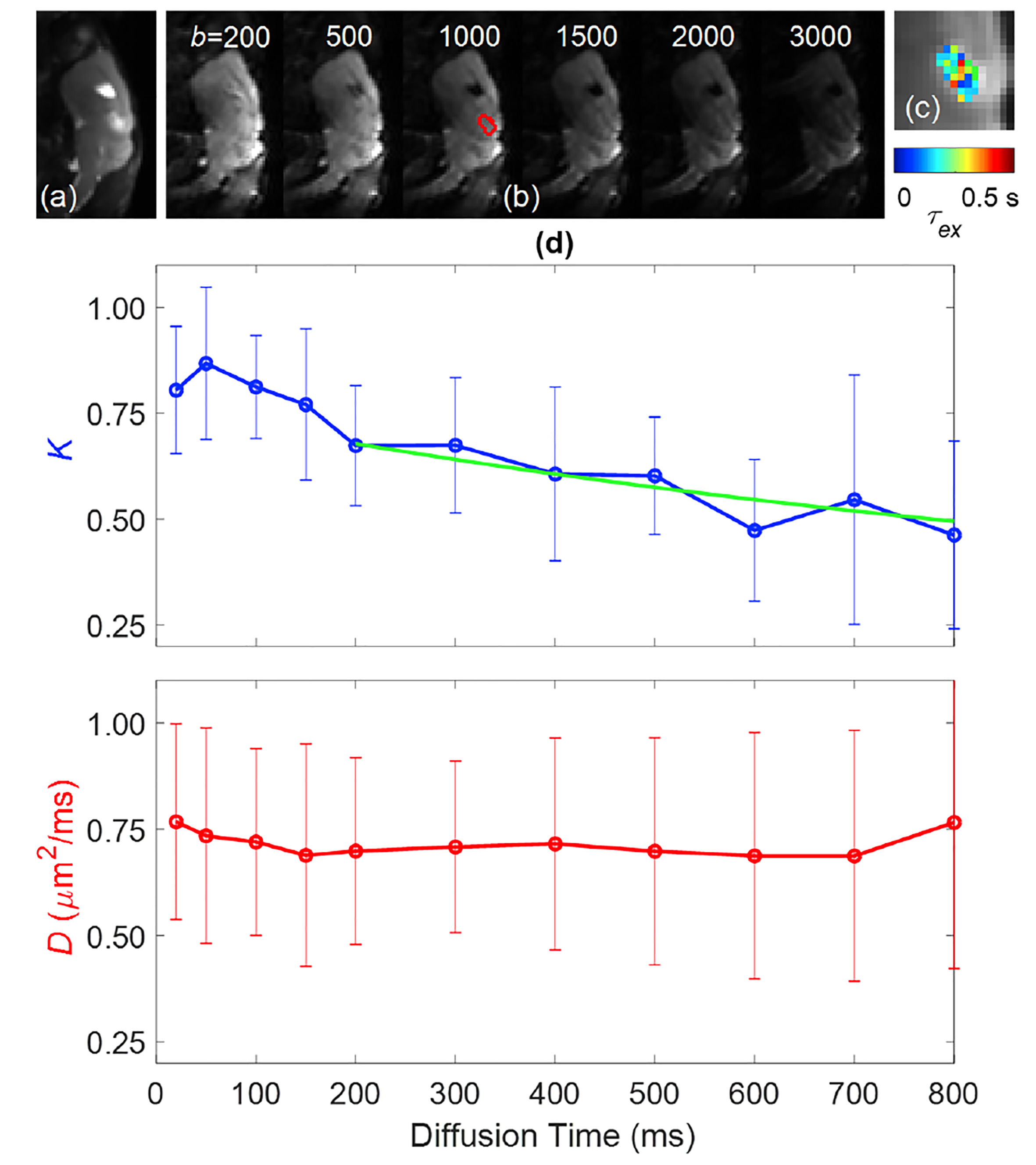
$$$\tau_{ex}$$$ from tDKI: dMRI measurement was conducted with multiple diffusion times between 20 and 800 ms while keeping the same b-values (b = 200, 500, 1000, 1500, 2000, 3000 s/mm2) by adjusting the diffusion gradient strength. tDKI data were acquired using a diffusion-weighted STEAM pulse sequence for tumor center slice (1 mm thickness) in sagittal direction with EPI readout (TR/TE = 8 s/30 ms, FOV = 20x20 mm, image matrix = 80x80, resolution = 0.25×0.25mm). tDKI data at each diffusion time t was used to estimate D(t) and K(t) using a weighted linear least-squares fit method. In the Kärger model (KM),4,5 the overall D=(1-ve)De+veDi=const, while K(t) depends on t $$K(t)=K_0\frac{2\tau_{ex}}{t}\left[1-\frac{\tau_{ex}}{t}\left(1-e^{-\frac{t}{\tau_{ex}}}\right)\right]+K_\infty\hspace{3em}[1]$$ with the exchange time $$$\tau_{ex}$$$=ve$$$\tau_i$$$=(1-ve)$$$\tau_e$$$, and K0 = 3$$$\frac{var\left(D\right)}{D^2}$$$, where $$$var$$$(D)=ve(1-ve)(Di-De)2. ve is interstitial volume fraction with $$$\tau_e$$$ denoting interstitial water lifetime. De and Di are extra- and intracellular diffusivities. The KM was applied for the data with long enough diffusion times where D(t) has already become constant, while K(t) is still decreasing solely because of the exchange, with a rate $$$1/\tau_{ex}$$$, Eq.[1].5 K$$$\infty$$$ accounts for tissue heterogeneity effects unrelated to exchange.
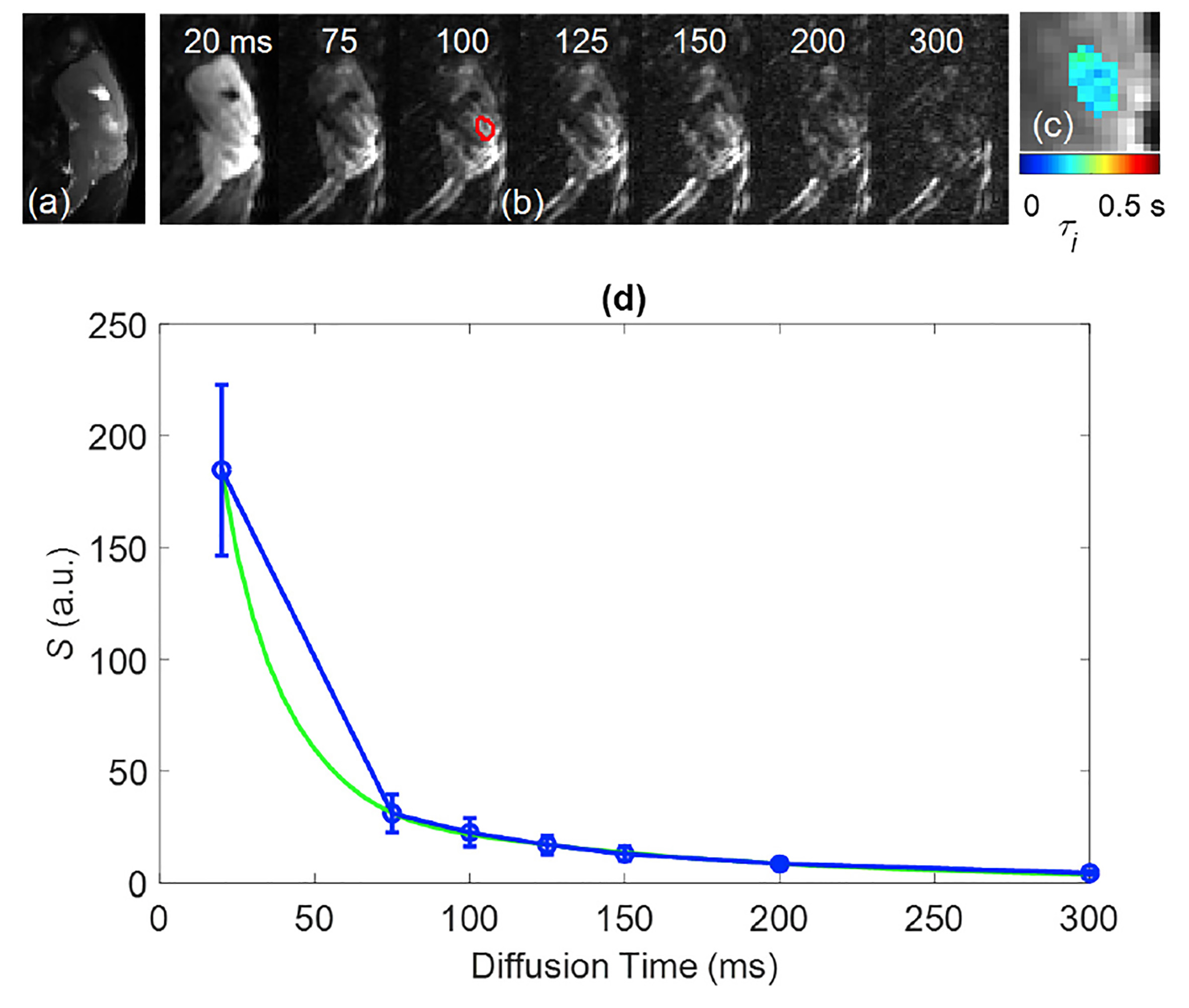
$$$\tau_i$$$ from CG-DWI: The same tumor center slice in the sagittal direction was also used for CG-DWI experiments with a STEAM-DWI sequence with TR/TE = 5 s/30 ms, diffusion gradient duration δ = 7 ms, and diffusion weighting gradient G = 150 mT/m. The sequence was run multiple times with a series of diffusion times; t = 20, 75, 100, 125, 150, 200 and 300 ms. Assuming extracellular signal contributions were dephased completely with the large q value when t is long enough, the intracellular water lifetime $$$\tau_i$$$, was determined by the monoexponential decay in long diffusion times.3 In order to avoid the need to select the lower bound of diffusion time for this analysis, a biexponential model was fit to the whole data set and the slow decay component was used to estimate $$$\tau_i$$$.
Results
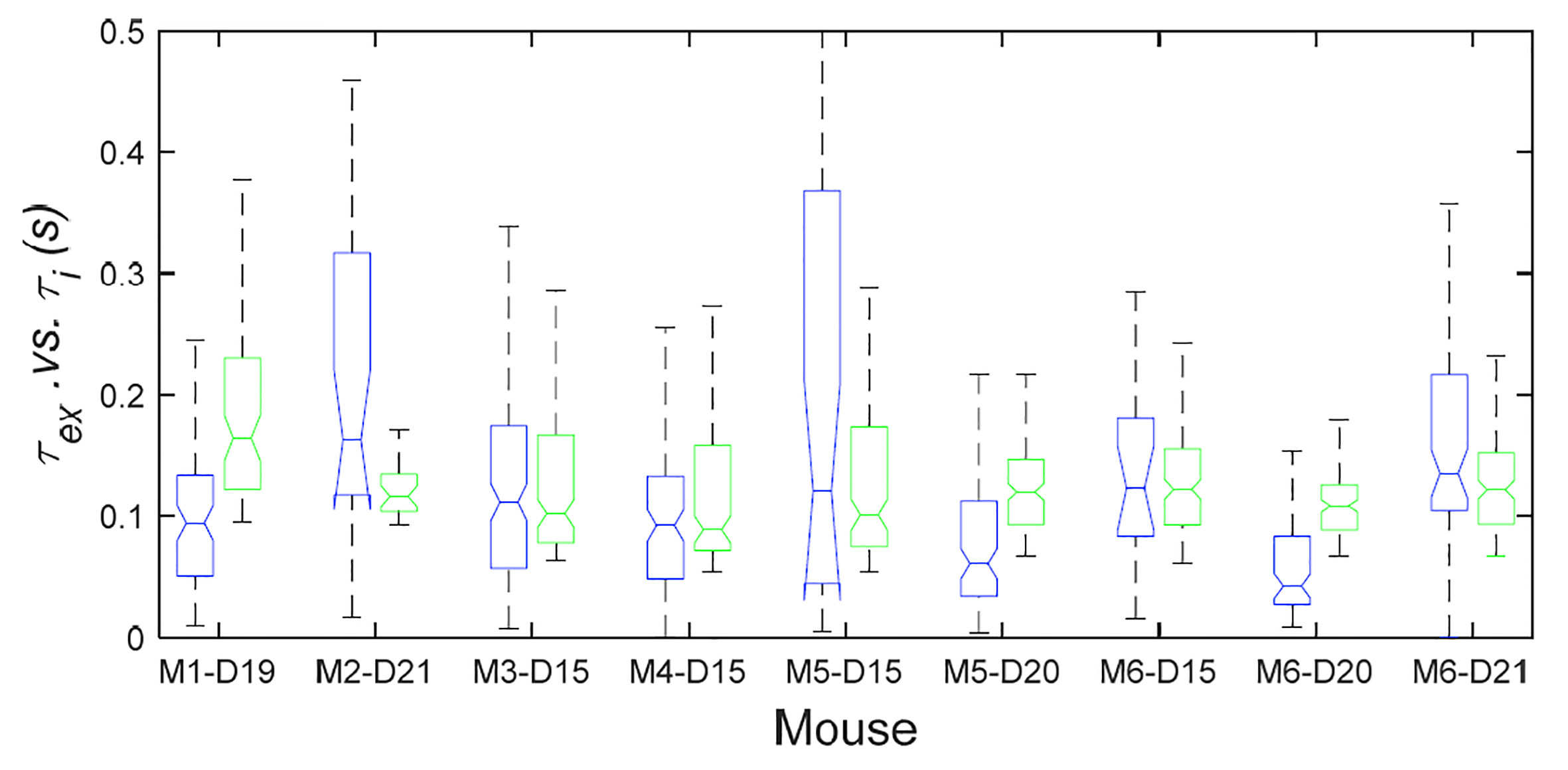
Figure 1 shows an example of D(t) and K(t) data acquired from a mouse with GL261 tumor. When t > 150 ms, D(t) does not show a noticeable change, while K(t) keeps decreasing monotonically. This is where the above condition to extend the KM to tissue microstructure becomes valid, such that Eq.[1] can be used to estimate $$$\tau_{ex}$$$. The fit shown in Figure 1d suggests that the water exchange time $$$\tau_{ex}$$$ = 111 ms, which is in the range expected for cancer cells.6 Figure 2 shows an example of the CG-DWI measurement for the same mouse shown in Figure 1. The slow component of a biexponential fit to the whole data points (Figure 2d) corresponded to the intracellular water lifetime of $$$\tau_i$$$ = 102 ms. Both $$$\tau_{ex}$$$ and $$$\tau_i$$$ measured in all six tumors, including multiple scans for two tumors, were in a similar range as shown in Figure 3.Discussion and Conclusion
The preliminary results from this study suggest that either of dMRI methods can be used to investigate the cellular-interstitial water exchange and its potential as a biomarker for tumor aggressiveness and treatment response. The CG-DWI method does not rely on a theoretical model, but requires using stronger diffusion weightings than the tDKI methods, which leads to lower signal-to-noise ratio in the data. It is expected that the tDKI method could be more easily applied in clinical applications.Acknowledgements
NIH R01CA160620, NIH R01CA219964, P41EB017183, NIH/NCI 5P30CA016087References
- Reynaud O. Time-Dependent Diffusion MRI in Cancer: Tissue Modeling and Applications. Front Phys 2017;5.
- Li H, Jiang X, Xie J, Gore JC, Xu J. Impact of transcytolemmal water exchange on estimates of tissue microstructural properties derived from diffusion MRI. Magn Reson Med 2017;77(6):2239-2249.
- Pfeuffer J, Flogel U, Dreher W, Leibfritz D. Restricted diffusion and exchange of intracellular water: theoretical modelling and diffusion time dependence of 1H NMR measurements on perfused glial cells. NMR Biomed 1998;11(1):19-31.
- Jensen JH, Helpern JA, Ramani A, Lu H, Kaczynski K. Diffusional kurtosis imaging: the quantification of non-gaussian water diffusion by means of magnetic resonance imaging. Magn Reson Med 2005;53(6):1432-1440.
- Fieremans E, Novikov DS, Jensen JH, Helpern JA. Monte Carlo study of a two-compartment exchange model of diffusion. NMR Biomed 2010;23(7):711-724.
- Springer CS, Jr., Li X, Tudorica LA, Oh KY, Roy N, Chui SY, Naik AM, Holtorf ML, Afzal A, Rooney WD, Huang W. Intratumor mapping of intracellular water lifetime: metabolic images of breast cancer? NMR Biomed 2014;27(7):760-773.
Figures