0970
Real-Time T1/PRF-Based MR Thermometry Using Deep Learning and VFA-mFFE for Guidance of HIFU Treatment1Department of Electronics and Information, Korea University, Seoul, Korea, Republic of, 2Korea Artificial Organ Center, Korea University, Seoul, Korea, Republic of, 3ICT Convergence Technology for Health and Safety, Korea University, Sejong, Korea, Republic of, 4Research Institute for Advanced Industrial Technology, Korea University, Sejong, Korea, Republic of, 5Bioimaging Research Team, Korea Basic Science Institute, Chungcheongbuk-do, Korea, Republic of, 6Correspoding author, ohch@korea.ac.kr, Seoul, Korea, Republic of
Synopsis
MR temperature mapping of adipose and aqueous tissues is crucial in ensuring the safety and efficacy of HIFU treatment in regions of the body where the adipose and aqueous tissues are treated. We suggest a simultaneous and real-time temperature mapping method for adipose and aqueous tissues by using deep learning and multi-echo fast field echo with
Introduction
MR temperature mapping of adipose and aqueous tissues is important to ensure the safety and efficacy of HIFU treatment for body regions where the adipose and aqueous tissues are treated. Although simultaneous acquisition methods of the temperatures of the adipose and aqueous tissues based on PRF and T1 has been proposed1,2, the methods are impractical for monitoring the thermal treatment because of the problems that PRF and T1 cannot be updated simultaneously with a single acquisition and the time for calculating T1 is long3. To overcome these limitations, we suggest a method of real-time and simultaneous update of the temperature of adipose and aqueous tissues using deep learning and multi-echo fast field echo with variable flip angle (VFA-mFFE)4. Additionally, to reconstruct the undersampled data obtained in the treatment stage, an image reconstruction method additionally using the high-resolution image obtained in the planning stage is proposed.Materials and Methods
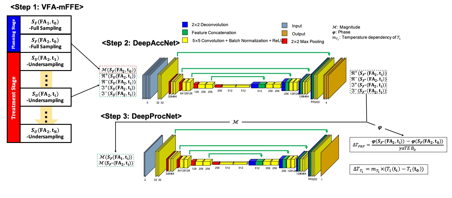
The data acquisition and image processing steps are as follows (Fig. 1):
Step 1.Data Acquisition (undersampled k-space and VFA-mFFE)
Step 1 is to acquire MR images. In this step, the fully-sampled complex MR images ($$$S_{F}(FA_{1},t_{0})$$$, $$$S_{F}(FA_{2},t_{0})$$$) are acquired with mFFE of several flip angles (FA’s) in the planning stage and undersampled complex MR data ($$$S_{U}(FA_{2},t_{i})$$$) is acquired with mFFE of a single flip angle in the treatment stage.
Step 2.Image Reconstruction (DeepAccNet)
Step 2 is the image reconstruction step accelerated by using deep learning. Five inputs are used. The input layer contains high-resolution MR magnitude image ($$$M(S_{F}(FA_{2},t_{0}))$$$) acquired in the planning stage of step 1. Therefore, the input layer consists of $$$M(S_{F}(FA_{2},t_{0}))$$$, $$$\Re ^{+} (S_{U}(FA_{2},t_{i}))$$$, $$$\Re ^{-} (S_{U}(FA_{2},t_{i}))$$$, $$$\Im ^{+} (S_{U}(FA_{2},t_{i}))$$$, and $$$\Im ^{-} (S_{U}(FA_{2},t_{i}))$$$. The output layer consists of $$$\Re ^{+} (S_{F^{*}}(FA_{2},t_{i}))$$$, $$$\Re ^{-} (S_{F^{*}}(FA_{2},t_{i}))$$$, $$$\Im ^{+} (S_{F^{*}}(FA_{2},t_{i}))$$$, and $$$\Im ^{-} (S_{F^{*}}(FA_{2},t_{i}))$$$. Here, $$$M(x)$$$ indicates the magnitude of $$$x$$$, and $$$\Re ^{+/-}(x)$$$ and $$$\Im ^{+/-}(x)$$$ represent the positive/negative real and imaginary values of $$$x$$$, respectively.
Step 3.Post-processing (DeepProcNet)
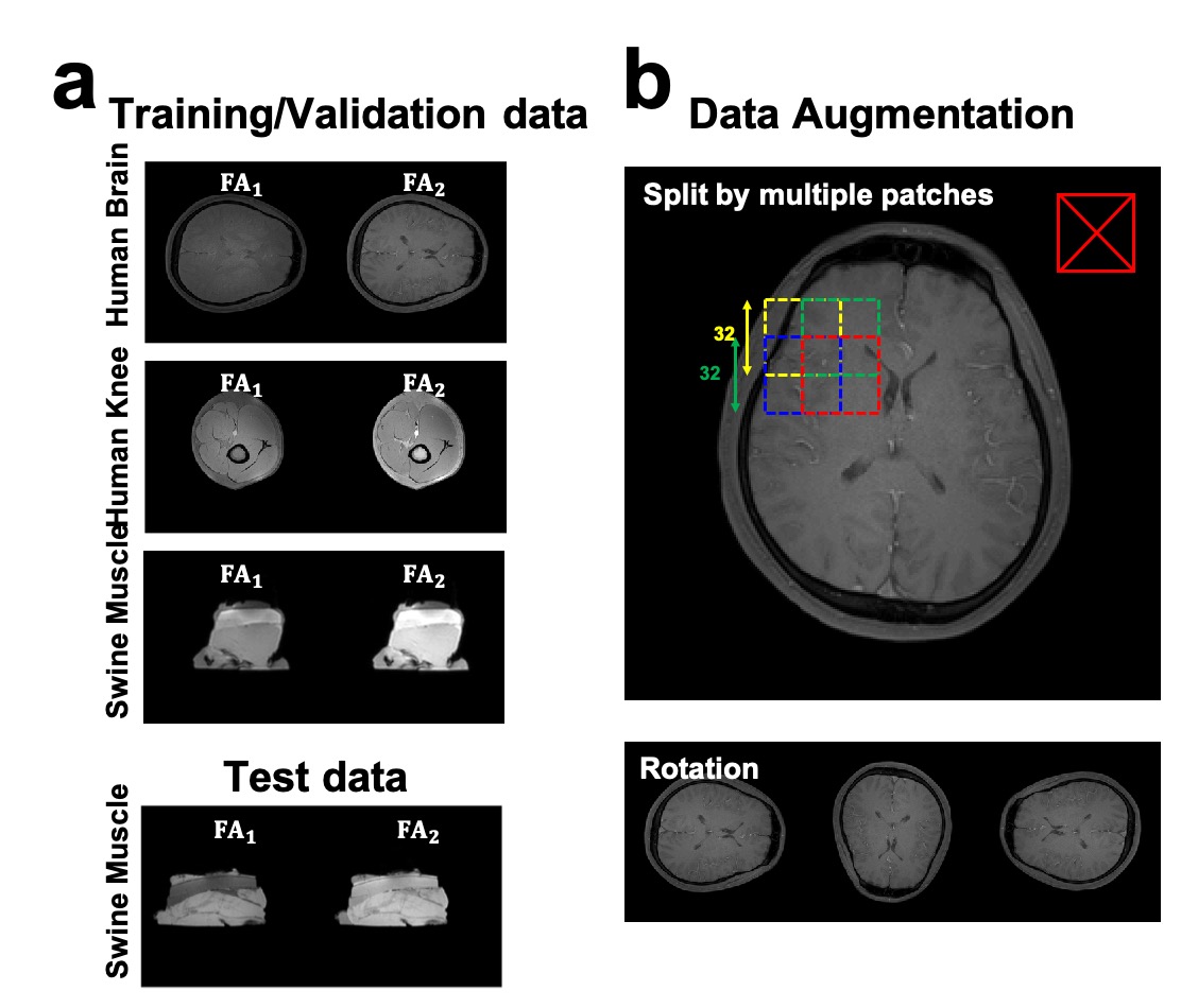
Step 3 is the step of T1 mapping using deep learning. The T1-based MR temperature is calculated by using deep learning from the magnitude images ($$$M(S_{F}(FA_{1},t_{0}))$$$, $$$M(S_{F^{*}}(FA_{2},t_{i}))$$$) of the image calculated in step 2, and the PRF-based MR temperature is calculated from the phase images ($$$\varphi (S_{F}(FA_{2},t_{0}))$$$, $$$\varphi(S_{F^{*}}(FA_{2},t_{i}))$$$). A 2-dimensional patch with the size of 32×32 voxels was used to increase the number of training set and flexibility of the network. The patch was generated with overlap of 50 %between adjacent patches (Fig. 2). Here, $$$\varphi(x)$$$ indicates the phase of $$$x$$$.
Data Acquisition and Training
The U-net architecture is used for deep neural networks5. Training and testing were conducted using Keras on a system equipped with a Nvidia GeForce GTX 1080TI GPU. 570 MR images from the knee and brain of three healthy volunteers and 95 dynamic scans of MR images from three swine muscle samples were also used in the process. MR data were acquired using VFA-mFFE on a 3-Tesla MRI scanner (Philips, Achieva, The Netherlands) equipped with a HIFU system (EfoE Ultrasonics, Inc., SouthKorea, center frequency=2.31MHz). MR parameters for HIFU treatment monitoring were as follows: Field-of-view: 192×1925 mm3, voxel size: 1×1×5 mm3, TR: 50 ms, TE’s: 3,5.6,8.2,10.8,13.4 ms, and flip angle: 10/35o. For performance evaluation of DeepAccNet, the acquired MR data is retrospectively undersampled by keyhole scheme with 48 encoding steps6.
Results and Discussion
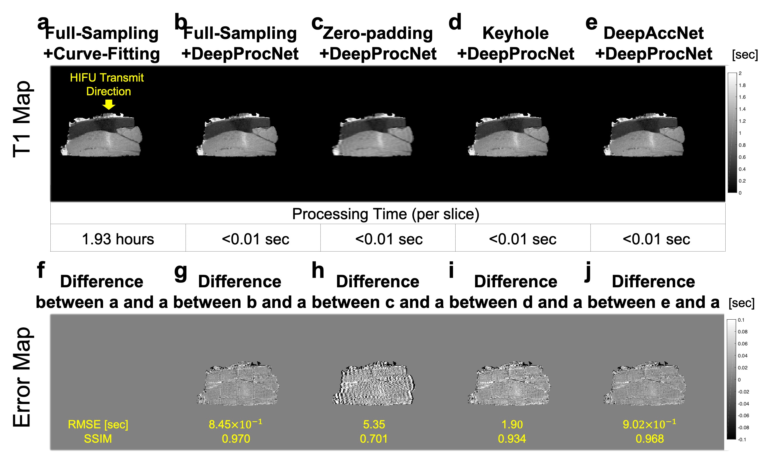
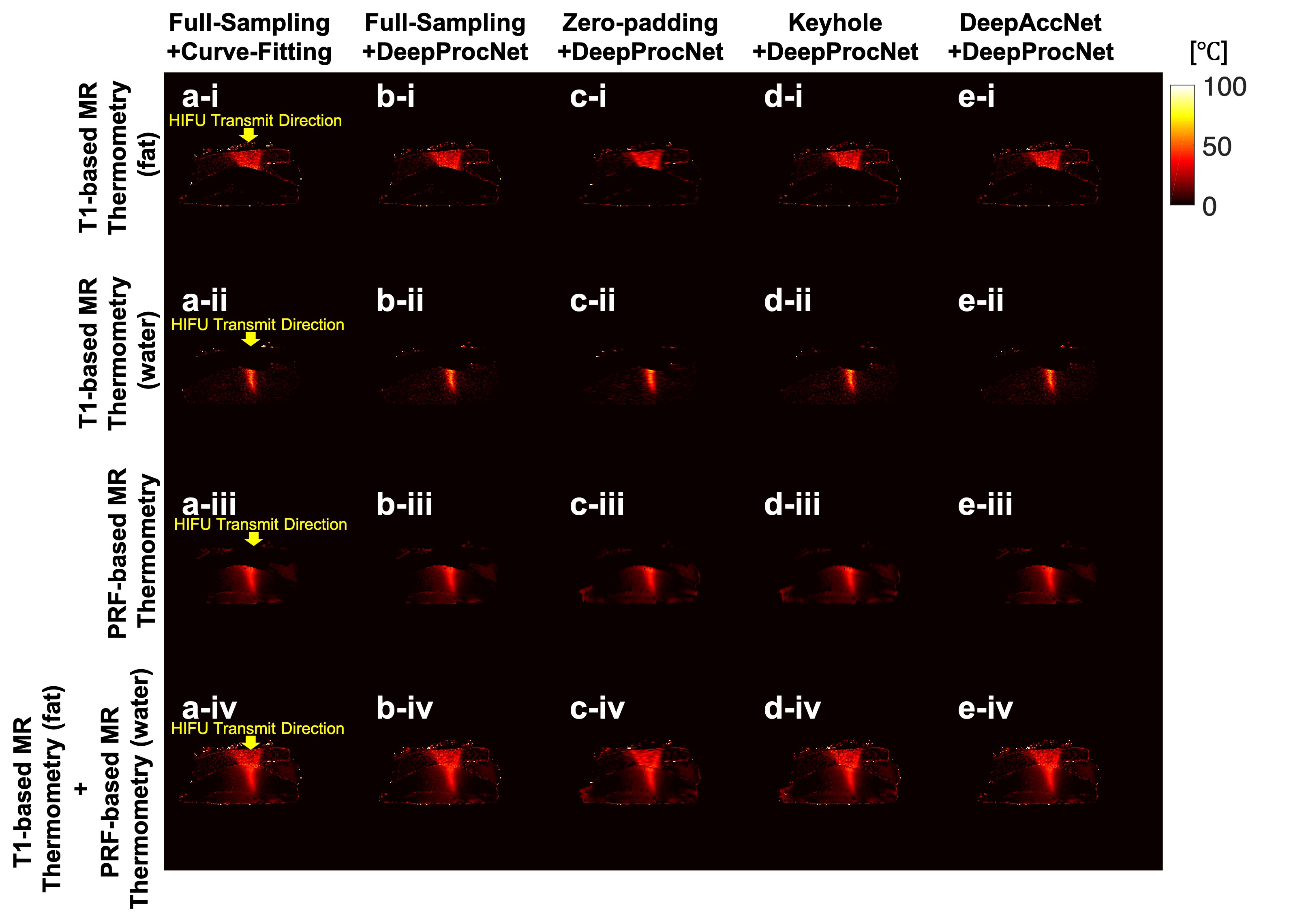
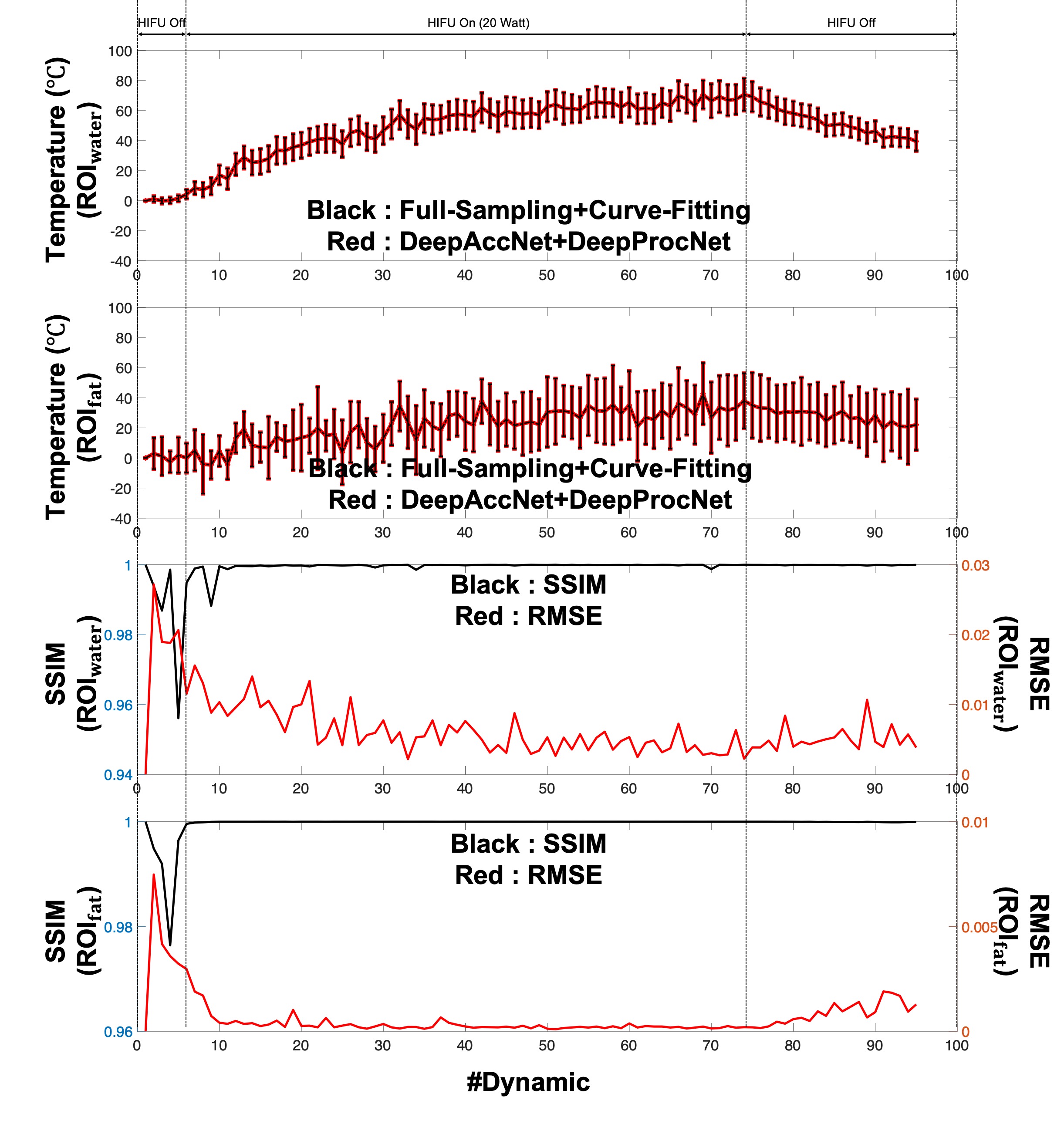
Figure 3 shows T1 maps from Full-Sampling+Curve-Fitting, Full-Sampling+DeepProcNet, Zero-padding+DeepProcNet, Keyhole+DeepProcNet, and DeepAccNet+DeepProcNet. The Root-Mean-Square-Error (RMSE) and Structural Similarity Index (SSIM) between T1 values of Full-Sampling+Curve-Fitting and Full-Sampling+DeepProcNet were 0.841 and 0.970, respectively. With 48 encodings, the RMSE and SSIM between T1 values of Full-Sampling+Curve-Fitting and DeepAccNet+DeepProcNet were very similar to those of Full-Sampling+Curve-Fitting and were better than those of Zero-padding+DeepProcNet and Keyhole+DeepProcNet. The processing time for Full-Sampling+DeepProcNet and DeepAccNet+DeepProcNet was less than 0.01 seconds, but that of Full-Sampling+Curve-Fitting was 1.2 hours. Figure 4 shows the representative examples of the temperature distribution from different methods. In the cases of Zero-padding+DeepProcNet and Keyhole+DeepProcNet, the image distortion was observed which was not noticed in the results of Full-Sampling+DeepProcNet and DeepAccNet+DeepProcNet. Figure 5 shows the mean, standard-deviation, SSIM, and RMSE between dynamic temperature variations of Full-Sampling+Curve-Fitting and DeepAccNet+DeepProcNet. During the dynamic scan, variations of the SSIM and RMSE were stable.Conclusions
In this study, we developed MR data acquisition, image processing, and post-processing methods to monitor the temperature distribution of adipose and aqueous tissues in real-time during thermal treatment. DeepAccNet is expected to be efficient not only in Keyhole but also in other acceleration methods7,8. Additional guidance and monitoring data such as magnetic susceptibility and electrical conductivity can also be calculated by mFFE data9.Acknowledgements
This work was supported by the Technology Innovation Program (#10076675) funded by the Ministry of Trade, Industry Energy (MOTIE, Korea).References
[1] Todd N, et al. Hybrid proton resonance frequency/T1 technique for simultaneous temperature monitoring in adipose and aqueous tissues. Magn Reson Med. 2013; 69(1): 62-70.
[2] Hey S, et al. Simultaneous T1 measurements and proton resonance frequency shift based thermometry using variable flip angles. Magn Reson Med. 2012; 67(2): 457-463.
[3] Kerr AB, et al. Real-time interactive MRI on a conventional scanner. Magn Reson Med. 1997; 38(3): 355-367.
[4] Cheng HL, et al. Rapid high resolution T1 mapping by variable flip angles: accurate and precise measurements in the presence of radiofrequency field inhomogeneity. Magn Reson Med. 2006; 55(3): 566-574.
[5] Ronneberger O, et al. U-net: Convolutional networks for biomedical image segmentation. International Conference on Medical image computing and computer-assisted intervention 2015; 234-241.
[6] Han YH, et al. Evaluation of the keyhole technique applied to the proton resonance frequency method for magnetic resonance temperature imaging. J Magn Reson Imag. 2011; 34(5): 1231-1239.
[7] Pruessmann, KP, et al. SENSE: sensitivity encoding for fast MRI. Magn Reson Med. 1999; 42(5): 952-962.
[8] Breuer FA, et al. Controlled aliasing in parallel imaging results in higher acceleration (CAIPIRINHA) for multi‐slice imaging. Magn Reson Med. 2005; 53(3): 684-691.
[9] Kim J-M, et al. Monitoring and Guidance on High-Intensity Focused Ultrasound Treatment by Multiple Fast Field Echo at 3.0 T MRI: Ex-Vivo Studies with Multiparametric Mapping. ISMRM 2018; 1485.
Figures