Synopsis

Low-dimensional subspace models have recently been developed for fast, high-SNR MRSI, by effectively reducing the degrees-of-freedom for the imaging problem. However, low-dimensional linear subspace models may be inadequate in capturing more complicated spectral variations across a general population. This work presents a new approach to model general spectroscopic signals, by learning a nonlinear low-dimensional representation. Specifically, we integrated the well-defined spectral fitting model and a deep autoencoder network to learn the low-dimensional manifold where the high-dimensional spectroscopic signals reside, and applied this learned model for denoising and reconstructing MRSI data. Promising results have been obtained demonstrating the potential of the proposed method.

INTRODUCTION

THEORY AND METHODS

Learning Low-Dimensional Representation for Spectroscopy Data

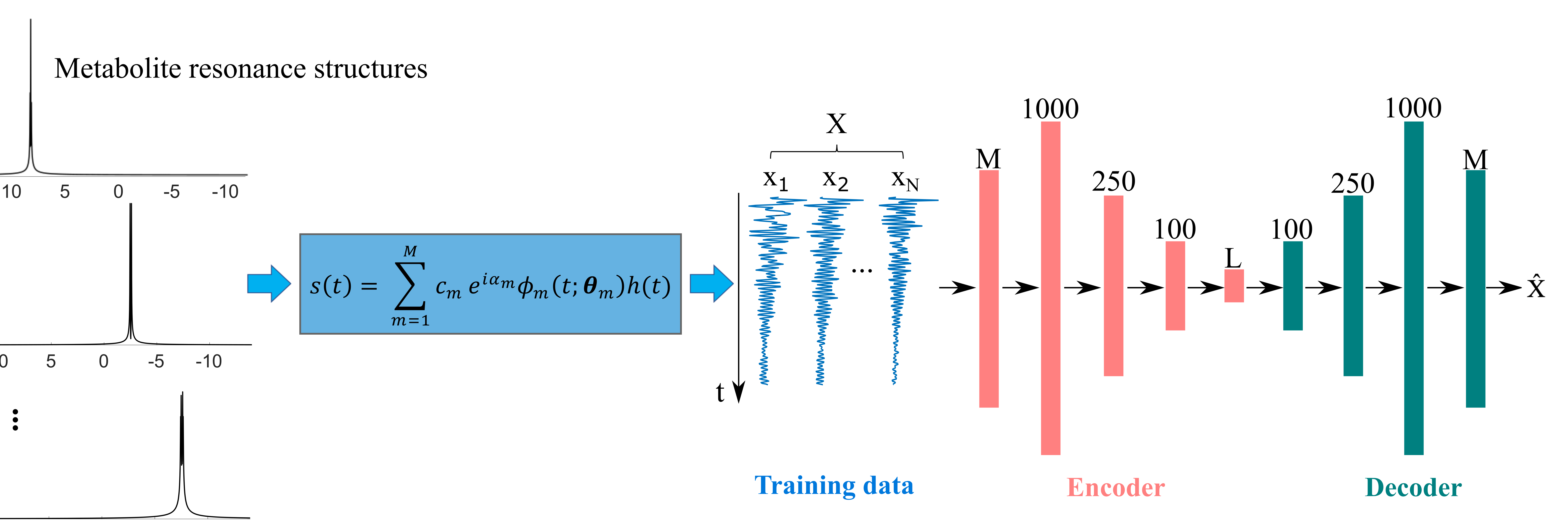
A general spectroscopy signal can be modeled as $$s(t)=\sum_{m=1}^Mc_me^{i\alpha_m}\phi_m(t;\boldsymbol{\theta}_m)h(t), \qquad\qquad\qquad\qquad\qquad\qquad\qquad\qquad [1]$$

where $$$\phi_m(t;\boldsymbol{\theta}m)$$$ represents the spectral variation for the $$$m$$$th molecule characterized by a resonance structure and molecule-dependent nonlinear parameters $$$\boldsymbol{\theta}_m$$$, $$$c_m$$$ denotes the concentrations, $$$\alpha_m$$$ the phases and $$$h(t)$$$ captures additional lineshape distortion (e.g., due to field inhomogeneity and eddy currents). Therefore, the ensemble of these signals reside in a nonlinear low-dimensional manifold⁸, which can be well-approximated by a linear subspace if the parameters are in a narrow range^5-7. However, as the ranges of $$$\theta_m$$$ and/or $$$M$$$ increase (for more complicated spectral variations), the linear subspace approximation becomes less accurate.

Meanwhile, learning a more general nonlinear representation of $$$\{s(t)\}$$$ is also challenging. Motivated by the recent success of deep learning and the well-define governing model for spectroscopic signals, we propose to use a deep autoencoder network (DAE)⁹ to address this problem. Specifically, we perform spectral fitting to a set of experimental MRSI data using Eq. [1], and apply random perturbations to the estimated parameters ($$$c_m$$$, $$$\alpha_m$$$, $$$\boldsymbol{\theta}_m)$$$ to generate a large collection of FID signals. This enabled the training of a DAE (Fig. 1) to learn a nonlinear low-dimensional representation of these signals, which can be used for general MRSI experiments.

Application of the Learned Model

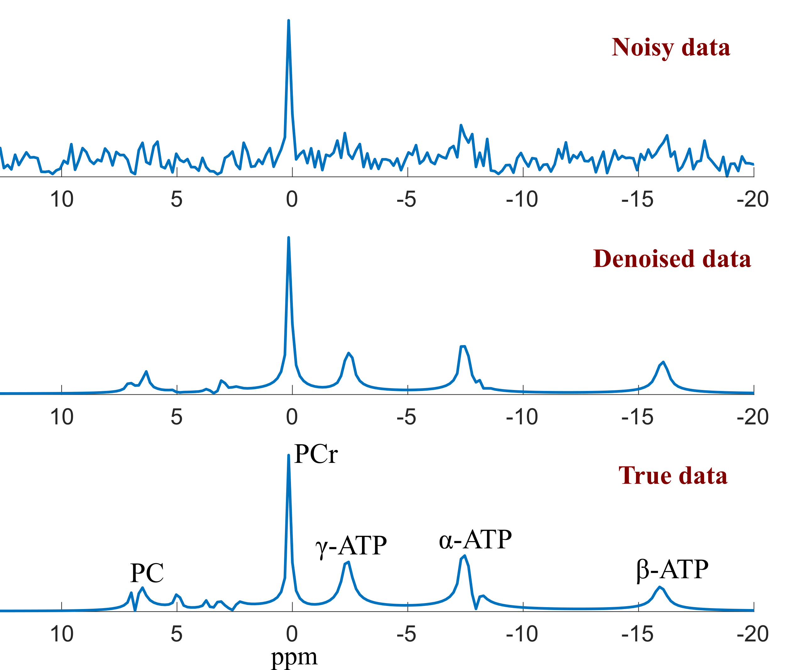
The learned nonlinear representation can be adapted for various MRSI processing tasks. We considered two examples here. The first one is to denoise single-voxel noisy spectra. More specifically, denoting the trained DAE as $$$P_{\mathbf{w}}(\cdot)$$$, the denoising can be done by passing the noisy data through $$$P_{\mathbf{w}}(\cdot)$$$, which projects the data onto the learned low-dimensional manifold for noise reduction.

The second example is reconstructing the desired spatiospectral function, denoted as $$$\mathbf{X}$$$, from noisy or sparse data. Such a problem can be formulated as

$$\hat{\mathbf{X}}=\arg\underset{\mathbf{X}}{\min}\left\Vert\mathbf{d}-\mathcal{F}_{\Omega}\{\mathbf{B}\odot\mathbf{X}\}\right\Vert_2^2+\lambda_1\left\Vert P_{\mathbf{w}}(\mathbf{X})-\mathbf{X}\right\Vert_F^2 +\lambda_2R(\mathbf{X}), \quad [2]$$

where $$$\mathbf{B}$$$ models B₀ inhomogeneity, $$$\mathcal{F}_{\Omega}$$$ the Fourier encoding operator with a sampling pattern $$$\Omega$$$, and $$$\mathbf{d}$$$ the (k,t)-space data. The first regularization term imposes the learned nonlinear low-dimensional representation of $$$\mathbf{X}$$$, and the second applies spatial constraints (e.g., a weighted-$$$\ell_2$$$ penalty or an $$$\ell_1$$$ penalty⁶). An iterative algorithm was designed to solve Eq. [2] by alternating between solving a least-squares subproblem and a propagation of the updated estimate through the DAE¹⁰. The details of the algorithm was omitted due to space constraint.

RESULTS

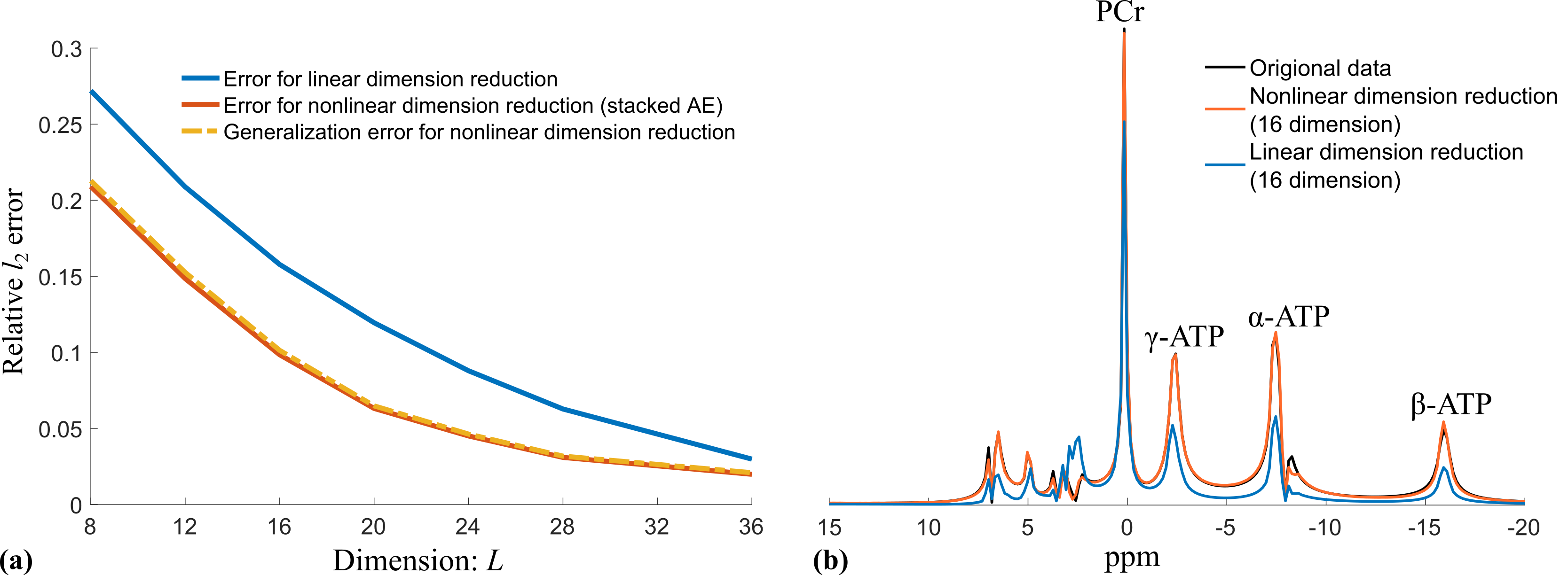
All simulations and experiments were based on brain ³¹P-MRSI data acquired on a 7T scanner (Siemens MAGNETOM), but note that the proposed methodology can also be applied to ¹H-MRSI or ¹³C-MRSI. We first evaluated the capability of the learned nonlinear representation for dimensionality reduction. Figure 2 compares the dimensionality reduction errors for the learned DAE and linear approximation (PCA). As can be seen, the learned DAE yielded higher accuracy than the linear subspace approximation, which is further confirmed by comparing the approximations for a fitted experimental in vivo ³¹P spectrum¹¹. Noise was then added to this data for a denoising test, and the results are shown in Fig. 3.

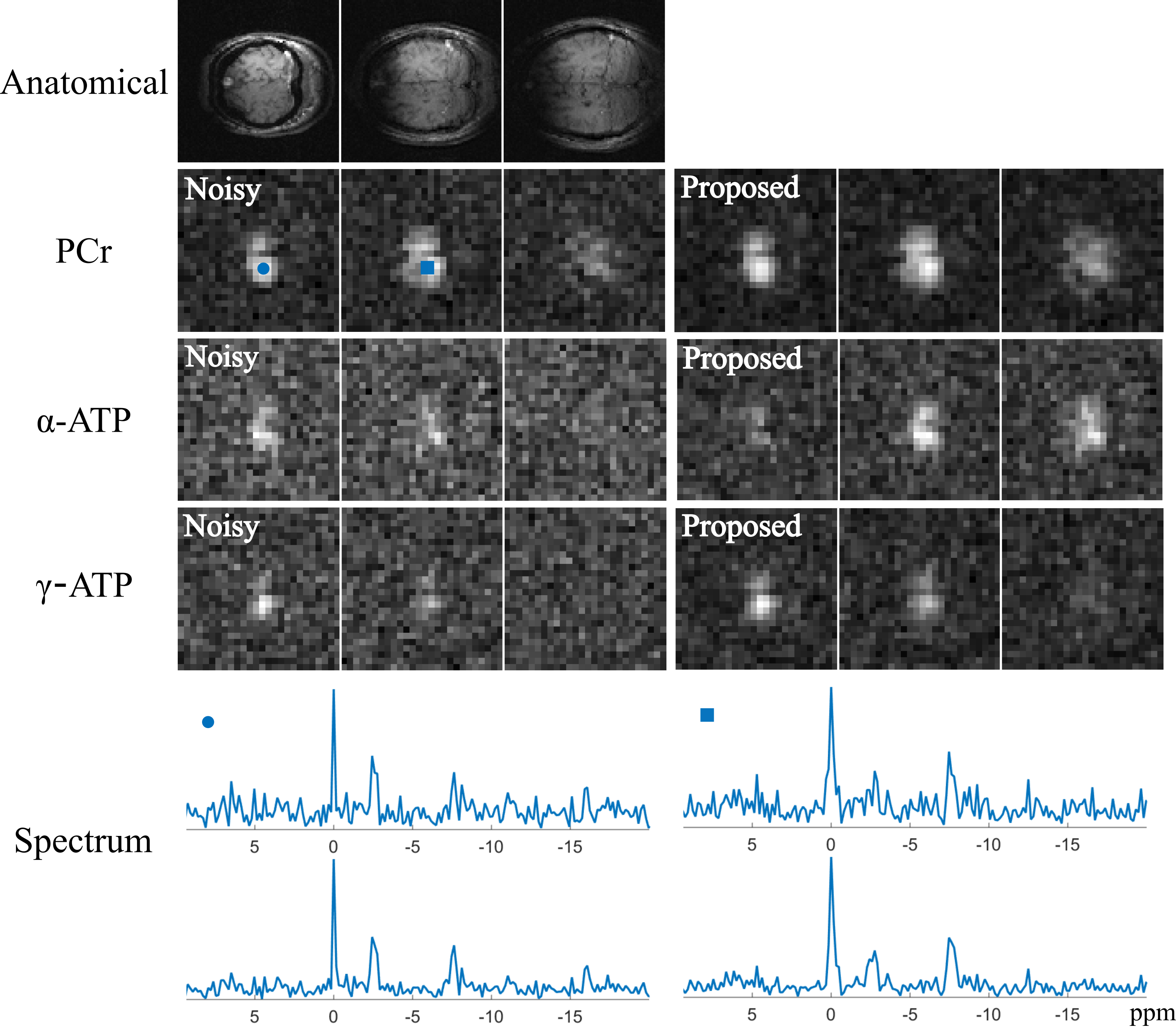
Figure 4 shows a spatiospectral reconstruction from a 3D ³¹P-CSI data. The improvement in SNR offered by the proposed reconstruction using learned DAE over standard Fourier reconstruction can be clearly observed, illustrated by the metabolite maps and the spatially-resolved spectra.

SUMMARY

Acknowledgements

References

1. Liang ZP and Lauterbur PC, A generalized series approach to MR spectroscopic imaging. IEEE Trans. Med. Imaging, 1991;10:132-137.

2. Haldar JP, Hernando D, Song S. and Liang ZP, Anatomically constrained reconstruction from noisy data. Magn. Reson. Med., 2008;59:810-818.

3. Eslami R and Jacob M, Robust reconstruction of MRSI data using a sparse spectral model and high resolution MRI priors, IEEE Trans. Med. Imaging, 2010;29:1297-1309.

4. Kasten J, Lazeyras F, and Van De Ville D, Data-driven MRSI spectral localization via low-rank component analysis. IEEE Trans. Med. Imaging, 2013;32:1853-1863.

5. Nguyen HM, Peng X, Do MN and Liang ZP, Denoising MR spectroscopic imaging data with low-rank approximations. IEEE Trans. Biomed. Eng., 2013;60:78-89.

6. Lam F, Ma C, Clifford B, Johnson CL, and Liang ZP, High‐resolution 1H‐MRSI of the brain using SPICE: Data acquisition and image reconstruction. Magn. Reson. Med., 2016;76:1059-1070.

7. Li Y, Lam F, Clifford B and Liang ZP, A subspace approach to spectral quantification for MR spectroscopic imaging. IEEE Trans. Biomed. Eng., 2017;64:2486-2489.

8. Yang G, Raschke F, Barrick TR and Howe FA, Manifold Learning in MR spectroscopy using nonlinear dimensionality reduction and unsupervised clustering. Magn. Reson. Med., 2015;74:868-878.

9. Hinton GE and Salakhutdinov RR, Reducing the dimensionality of data with neural networks. Science, 2006;28:504-507.

10. Aggarwal HK, Mani MP and Jacob M, Model based image reconstruction using deep learned priors (MODL), IEEE-ISBI 2018, pp. 671-674.

11. Deelchand DK, Nguyen TM, Zhu XH, Mochel F and Henry PG, Quantification of in vivo 31P NMR brain spectra using LCModel. NMR Biomed., 2015;28:633-641.