Synopsis

Gradient impulse response function (GIRF) can be used to characterize gradient systems. GIRF measurements typically require multiple triangular waveforms of different durations to be played in three gradient axes. Using the traditional method, the entire measurement takes more than 10 hours. In this study, we propose an interleaved off-isocenter method to measure GIRFs. It can save nearly 50% of measurement time. The measured results are consistent with those measured using the time-consuming traditional method.

Introduction

Methods

(i) Experiment parameters

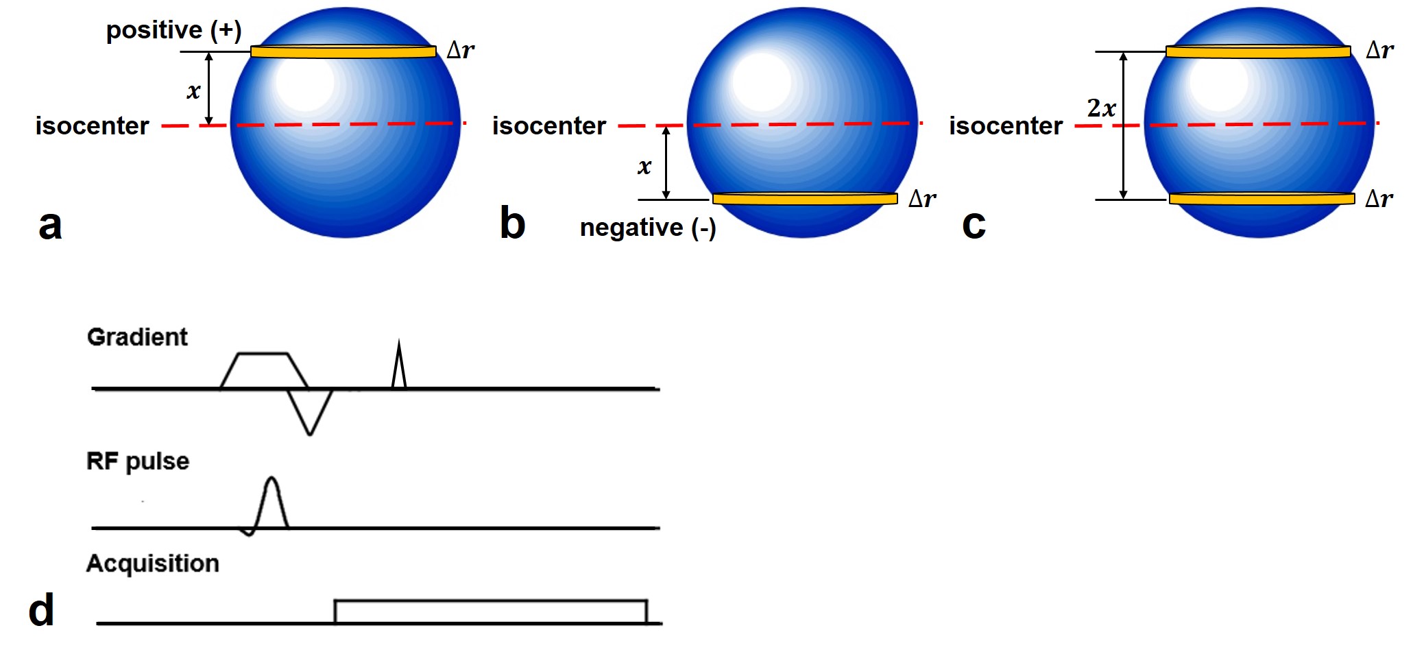
All experiments were performed on a Philips Achieva 3.0T MR system. GIRF measurements were implemented in two parallel slices (3mm thickness, 33mm apart) of a spherical phantom (Fig.1c). These two slices were a positive slice (+) at a distance of +16.5mm from the isocenter (Fig.1a) and a negative slice (-) at a distance of -16.5mm from the isocenter (Fig.1b), respectively. Twelve triangular waveforms with slew rate of 180mT/m/ms and durations from 0.10ms to 0.32ms were played out along the same axis as the slice-selective gradient respectively. Reference scans were obtained in the absence of these known inputs to eliminate eddy current contributions from the slice-selective gradient. The actual output gradient waveforms were calculated according to the phase variations of the measured FID signals. The sequence diagram of GIRF measurement is shown in Fig.1d. Considering the lifetime of FID signal and the eddy current induced by slice-selection gradient, the triangular gradients were applied over 1.4ms after slice-rephasing gradient. The acquisition started before the beginning of the test gradients to prevent the effects of acquisition delay on the output measurement. Other parameters were: TR=8s, flip angle=90°, readout=10ms, dwell time=8.5 μs, sampling bandwidth=118 kHz, 60 averages.

(ii) Measurement methods

1. Traditional approach [2,5]. The aforementioned two parallel slices were excited sequentially. After measuring in the positive slice (+), the same gradient needed to be tested again in the negative slice (-). The complete measurement took about 10.4h, T=8s×2slices×(12+1)×3dirs×60avg=10.4h.

2. Single-slice method [6]. The measurements can be performed in either the positive slice (+) or the negative slice (-). Then the measurements from one side were used for gradient calculation. Thus T=8s×1slice×(12+1)×3dirs×60avg=5.2h.

3. Proposed interleaved off-isocenter method. The positive slice (+) and the negative slice (-) were excited alternately. The same test gradient was played out only once. The odd test gradients were played in the positive slice (+) while the even gradients were played in the negative slice (-). Thus T=8s×2interleaves×(12/2+1)×3dirs×60avg=5.6h.

(iii) Validation

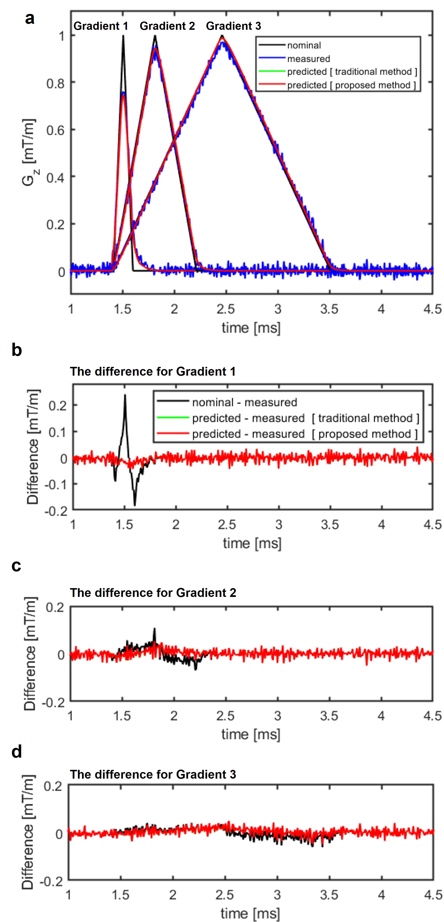
To validate the measured GIRFs using the traditional method and proposed method, the GIRFs were used to predict the gradient output. A comparison was made between the predicted gradient waveforms and measured gradients. The gradients used for validation were triangular waveforms (duration=0.2ms, 0.8ms and 2.1ms, amplitude=1 mT/m). These parameters were determined according to the reference 3.

Results and Discussion

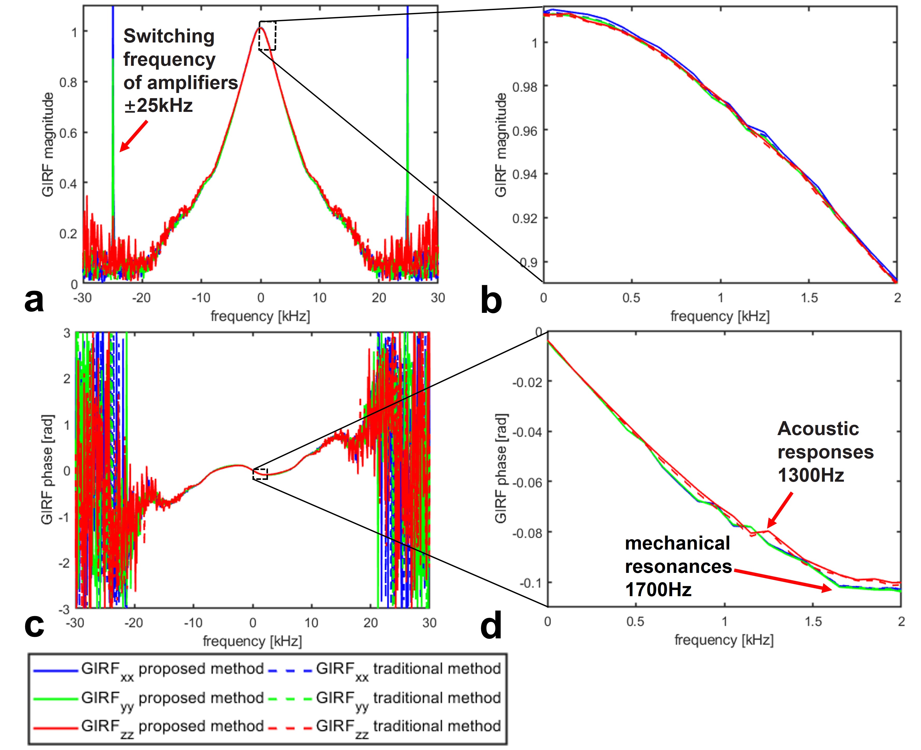
Magnitude and phase plots of the measured GIRFs along three gradient axes using traditional method and the proposed method are shown in Fig.2. It demonstrates that gradient chains have low-pass characteristics. Besides, the GIRF peaks at ±25kHz reflect the transistor switching frequency of gradient amplifiers, which is consistent with the results obtained using field probes [3]. At low frequency, the peaks around 1300Hz and 1700Hz are caused by acoustic responses and mechanical resonances of gradient coils, respectively. The measured GIRFs using our proposed method are consistent with those measured using the traditional method.

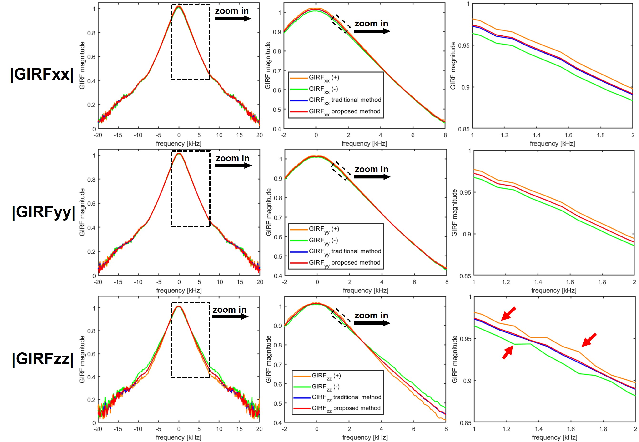
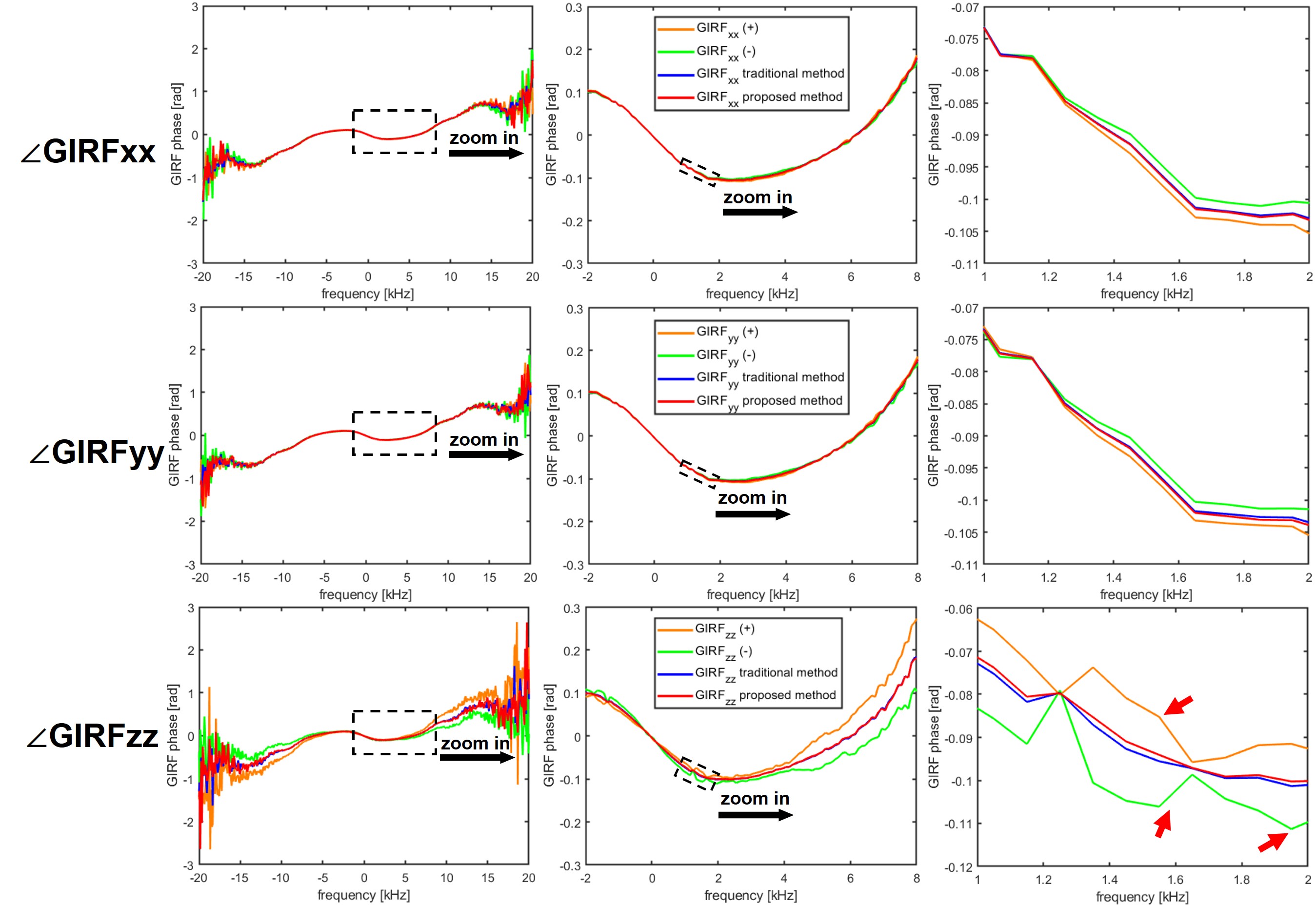
For further comparison, the magnitude and phase of the measured GIRFs using positive (+) single-slice method, negative (-) single-slice method, traditional method and proposed method are shown in Fig.3 and Fig.4, respectively. GIRF measurements using single-slice method [6] ignore the effect of main magnetic field drift, resulting in measurement results skewing and fluctuations in z direction. In contrast, the effect can be eliminated by measuring the same test gradient in two sides using the traditional method. GIRF measurements using our proposed method also can cancel the effect and save nearly 50% of measurement time. There is almost no difference between measured GIRFxx and GIRFyy using traditional method and our proposed method. The difference between measured GIRFzz is subtle.

As shown in Fig.5, the GIRF-based predictions are compared with nominal gradients and actual measured gradient waveforms. For shorter and steeper gradients, the differences between the actual and the nominal gradients are much larger than them in longer gradients.

Although there is subtle difference between measured GIRFzz using traditional method and the proposed method, the predicted values are extremely close.

Conclusion

Acknowledgements

References

[1] BRODSKY E K, SAMSONOV A A, BLOCK W F. Characterizing and correcting gradient errors in non‐cartesian imaging: are gradient errors linear time‐invariant (LTI)? [J]. Magnetic Resonance in Medicine: An Official Journal of the International Society for Magnetic Resonance in Medicine, 2009, 62(6): 1466-76.

[2] CAMPBELL‐WASHBURN A E, XUE H, LEDERMAN R J, et al. Real‐time distortion correction of spiral and echo planar images using the gradient system impulse response function [J]. Magnetic resonance in medicine, 2016, 75(6): 2278-85.

[3] VANNESJO S J, HAEBERLIN M, KASPER L, et al. Gradient system characterization by impulse response measurements with a dynamic field camera [J]. Magnetic resonance in medicine, 2013, 69(2): 583-93

[4] VANNESJO S J, DUERST Y, VIONNET L, et al. Gradient and shim pre-emphasis by inversion of a linear time-invariant system model [J]. Magnetic resonance in medicine, 2017, 78(4): 1607-22.

[5] STICH M, WECH T, SLAWIG A, et al. Gradient waveform pre-emphasis based on the gradient system transfer function [J]. Magnetic resonance in medicine, 2018

[6] LATTA P, GRUWEL M L, VOLOTOVSKYY V, et al. Simple phase method for measurement of magnetic field gradient waveforms [J]. Magnetic resonance imaging, 2007, 25(9): 1272-6.